Page 158 - Contributed Paper Session (CPS) - Volume 2

CPS1488 Willem van den B. et al.
2. Methodology
Let { } denote a partition of {1,...,n} into K ≥ 1 parts such that
=1

=1
={1,….,n} and Sj ∩Sk =∅ for j 6= k. Denote the number of elements in Sk
by nk = |Sk|. Let ySk denote the nk dimensional vector obtained by selecting the
elements from y with indices in Sk. Since the observation errors in (1) are
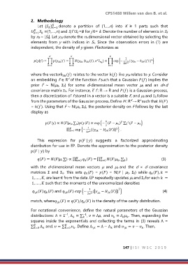
independent, the density of y given f factorizes as

1
2 ()|| }
2
(|) = ∏ ( |) = ∏ { |ℎ (), } ∝ ∏ exp {− 2 || − ℎ
2
=1 =1 =1

where the vectorℎ () relates to the vector ℎ() like ySk relates to y. Consider

d
an embedding F ∈ R of the function f such that a Gaussian () implies the
prior F ∼ N(µ0, Σ0) for some d-dimensional mean vector µ0 and an d×d
covariance matrix Σ0. For instance, if f : R → R and () is a Gaussian process,
then a discretization of f stored in a vector is a suitable F, and µ0 and Σ0 follow
d
from the parameters of the Gaussian process. Define H : R → R such that ()
n
= ℎ(). Using that F ∼ N(µ0, Σ0), the posterior density on F follows by the last
display as

1
(|) ∝ (| , ∑ )(|) ∝ exp {− ( − ) ∑ ( − }
−1

0
0
0
0
2 0
2
∏ exp {− 2 1 2 || − ()|| } .

=1

This expression for ( | ) suggests a factorized approximating
distribution for use in EP. Denote the approximation to the posterior density
( | ) by
() = (|, ∑) ∝ ∏ () = ∏ (| , ∑ ) (3)
=0

=0

with the d-dimensional mean vectors µ and µk and the d × d covariance
matrices Σ and Σk. This sets () = () = N(F | µ0, Σ0) while (), =
0

1, . . . , , are learnt from the data. EP repeatedly updates µk and Σk for each =
1, . . . , such that the moments of the unnormalized densities
1 2
() () and () {− || − ()|| } (4)

\
\

2 2
match, where () ∝ ()/ () is the density of the cavity distribution.

\
For notational convenience, define the natural parameters of the Gaussian
−1
distributions: Λ = Σ , Λ = ∑ , = Λ, and = µ . Then, expanding the
−1

squares inside the exponentials and collecting the terms in (3) reveals Λ =
∑ Λ and. = ∑ . Define Λ \ = Λ − Λ and \ = − . Then,
=0

=0

147 | I S I W S C 2 0 1 9