Page 207 - Contributed Paper Session (CPS) - Volume 2

CPS1824 Sanggi L.
where ℎ1,⋯ , ℎ are the constituent households in wave 1 which jointly form
the new household at a later wave, and where 1, ⋯ , are the corresponding
selection probabilities. Because the wave 1 selection probabilities are only
known for respondents that were actually sampled and not for those
respondents that later joined into existing households, the following two
approaches are discussed to approximate it.

(The shared weights approach)
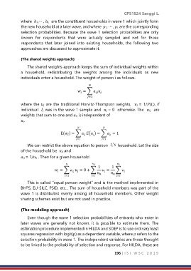
The shared weights approach keeps the sum of individual weights within
a household, redistributing the weights among the individuals as new
individuals enter a household. The weight of person i as follows.

= ∑

=1

where the are the traditional Horvitz-Thompson weights, = 1/(), if
individual was in the wave 1 sample and = 0 otherwise. The are
weights that sum to one and is independent of
.

We can restrict the above equation to person household. Let the size
of the household be ℎ and
= 1/ℎ . Then for a given household

This is called “equal person weight” and is the method implemented in
BHPS, EU-SILC, PSID, etc... The sum of household members was part of the
wave 1 is distributed evenly among all household members. Other weight
sharing schemes exist but are not used in practice.

(The modeling approach)
Even though the wave 1 selection probabilities of entrants who enter in
later waves are generally not known, it is possible to estimate them. The
estimation procedure implemented in HILDA and SOEP is to use ordinary least
squares regression with logit(p) as a dependent variable, where p refers to the
selection probability in wave 1. The independent variables are those thought
to be linked to the probability of selection and response. For HILDA, these are

196 | I S I W S C 2 0 1 9