Page 238 - Contributed Paper Session (CPS) - Volume 2

CPS1845 Devni P.S. et al.

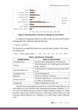
PAUH
PADANG_UTARA
PADANG_TIMUR
PADANG_BARAT
Weight
NANGGALO
Medium
LUBUK_BEGALUNG
Slight
KURANJI
KOTO_TANGAH
BUNGUS_TELUK_KABUNG

0 1000 2000 3000 4000 5000 6000 7000 8000

Figure 2. Summary data on the level of damage for each District

To create and manipulate DAGs in the BN context, we will use the bnlearn
package (short for "Bayesian network learning").

> library (bnlearn)
The first step, we make DAG where one node for each variable in the survey
and without arc.

> dag <- empty.graph (node = c ("C", "P", "E", "L", "S", "F", "D"))
Table 3. Classification of Variables
Variable Release States or Intervals (unit)
Construction (C) Wood (1), Semi Permanent (2), Permanent (3)
86.19-90.89 gal (1), 91.11-93.99 gal (2), 94.27-96.94
PGA (P)
gal (3) >96.94 (4)
51.62-59.62 km (1), 59.78-64.22 km (2), 64.56-70.09
Epicenter distance (E)
km (3)
Landslide risk (L) Low (1), Moderate (2)
Slope (S) 0-2% (1), 2-15% (2), 15-40% (3)
15164.33-22683.49 km (1), 23574.32-29712.09 km
Close to faults (F)
(2), 29813.73-35780.49 km (3)
Damage (D) Slight (1), Moderate (2), Heavy (3)

The DAG is an empty graph, because the arc set is still empty. Now we can
start adding arcs that describe direct dependencies between variables. C, F, S,
and E are not influenced by any other variable. Therefore, there is no single
bow that leads to one variable. However, F and S have a direct effect on L and
E having a direct influence on P. Likewise, C, F, L, and P have a direct influence
on D.

227 | I S I W S C 2 0 1 9