Page 131 - Contributed Paper Session (CPS) - Volume 3

CPS1970 Nurul Aityqah Y. et al.
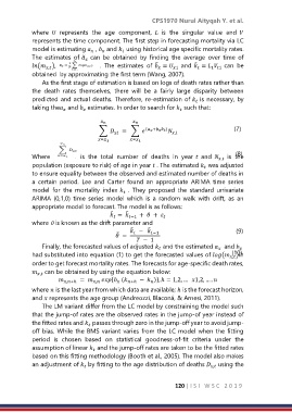
where represents the age component, is the singular value and
represents the time component. The first step in forecasting mortality via LC
model is estimating , and using historical age specific mortality rates.

The estimates of ̃ can be obtained by finding the average over time of

̃
̃
( ), . The estimates of = and = can be

1 1
,
1

obtained by approximating the first term (Wang, 2007).
As the first stage of estimation is based on logs of death rates rather than
the death rates themselves, there will be a fairly large disparity between
predicted and actual deaths. Therefore, re-estimation of is necessary, by

taking the and estimates. In order to search for such that:

∑ = ∑ ( + ) (7)

,
= 1 = 1
(8)
Where is the total number of deaths in year and is the
,
population (exposure to risk) of age in year . The estimated was adjusted

to ensure equality between the observed and estimated number of deaths in
a certain period. Lee and Carter found an appropriate ARIMA time series
model for the mortality index . They proposed the standard univariate

ARIMA (0,1,0) time series model which is a random walk with drift, as an
appropriate model to forecast. The model is as follows:
̃
̃
= −1 + +

where  is known as the drift parameter and
̃
̃
− −1 (9)

̃
=
− 1
Finally, the forecasted values of adjusted and the estimated and

(10)
had substituted into equation (1) to get the forecasted values of ( )in
,
order to get forecast mortality rates. The forecasts for age-specific death rates,
can be obtained by using the equation below:
,
,+ℎ = , { ( +ℎ − )}, ℎ = 1,2, … 1,2, … .

where is the last year from which data are available; ℎ is the forecast horizon,
and represents the age group (Andreozzi, Blaconá, & Arnesi, 2011).
The LM variant differ from the LC model by constraining the model such
that the jump-of rates are the observed rates in the jump-of year instead of
the fitted rates and passes through zero in the jump-off year to avoid jump-

off bias. While the BMS variant varies from the LC model when the fitting
period is chosen based on statistical goodness-of-fit criteria under the
assumption of linear and the jump-off rates are taken to be the fitted rates

based on this fitting methodology (Booth et al., 2005). The model also makes
an adjustment of by fitting to the age distribution of deaths using the

,
120 | I S I W S C 2 0 1 9