Page 229 - Contributed Paper Session (CPS) - Volume 3

CPS2002 Atina A. et al.
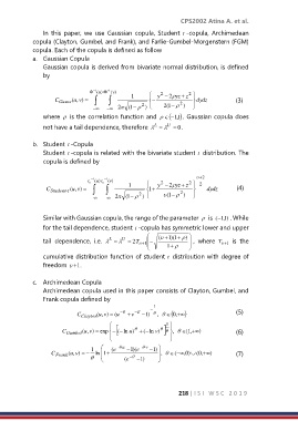
In this paper, we use Gaussian copula, Student t -copula, Archimedean
copula (Clayton, Gumbel, and Frank), and Farlie-Gumbel-Morgenstern (FGM)
copula. Each of the copula is defined as follow
a. Gaussian Copula
Gaussian copula is derived from bivariate normal distribution, is defined
by

−1
−1
)
 ( u  ( v) 1  y − 2 yz + z 

2
2
v =
 −
,
C Gauss ( u )    2  dydz (3)


−  −  2 1 ( −  2 )  1 ( 2 −  ) 
where  is the correlation function and  ( 1 . Gaussian copula does
−

) 1 ,
not have a tail dependence, therefore  L =  U = 0.

b. Student t -Copula
Student t -copula is related with the bivariate student t distribution. The
copula is defined by

 +2
t  −1 ( u t )  −1 ( v)  y − 2 yz + z 
2
2
 2
 +
v =
,
C Student t − ( u )   1  1 2  dydz (4)


−  −  2 1 ( −  2 )  1 (  −  ) 

Similar with Gaussian copula, the range of the parameter  is (− ) 1 , 1 . While
for the tail dependence, student t -copula has symmetric lower and upper
 (  1 1 + ) 
+ )(
tail dependence, i.e.  L =  U = 2T  +1   −   , where T  1 + is the
 1 +  
cumulative distribution function of student t distribution with degree of

freedom + 1.

c. Archimedean Copula
Archimedean copula used in this paper consists of Clayton, Gumbel, and
Frank copula defined by
1
−
( +
C Clayton (u , ) v = (u − + v − − ) 1  ,   , 0 ) (5)
 1 



(−
C Gumbel (u ,v ) = exp  −  ln u ) + (− ln ) v      , 1 [ + ) (6)
,

 


1  (e − u − 1 )(e − v − ) 1 
C Frank (u ,v ) = −  ln    1+ (e − − ) 1    ,   (− ) 0 ,  , 0 ( + ) (7)
218 | I S I W S C 2 0 1 9