Page 230 - Contributed Paper Session (CPS) - Volume 3

CPS2002 Atina A. et al.
L
where Clayton has lower tail dependence  = 2  / 1 − , Gumbel has upper
U
tail dependence  = 2− 2 −  / 1 , and Frank does not have tail dependence
 L =  U = 0.
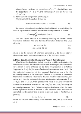
d. Farlie-Gumbel-Morgenstern (FGM) Copula
The bivariate FGM copula is defined by

C FGM (u ,v ) = uv + u 1 ( −u ) v 1 ( − v ),   [− ] 1 , 1 (8)

Parameter estimation of copula function is obtained by maximizing the
value of log-likelihood function with respect to the parameter as follows
n
ˆ
 = arg max  ln [ c ( F ( x ), F ( y ))] (9)
 X i Y i
= i 1
The best copula function is obtained by selecting the smallest Akaike
Information Criterion (AIC) and Bayesian Information Criterion (BIC) value
given by

AIC = 2k − 2 ln (L ˆ ) (10)
BIC = ln(n )k − 2 ln (L ˆ ) (11)

where k be the number of estimated parameters, n be the number of
ˆ
observations, and L be the maximum value of the likelihood function.

2.2 Yield-Based Agricultural Losses and Value at Risk Estimation
After fitting the distribution for both marginal variables and selecting the
best copula function, the estimation of the yield-based agricultural losses and
value at risk in terms of losses can be done. The procedure is as follows.
ˆ
ˆ
ˆ
ˆ
Suppose that  =  , k ˆ  , ˆ  be a set of estimated parameters where  and k be
ˆ
the estimated parameters of the marginal distributions and  be the
estimated parameter of the best copula function. Suppose that X represents
the weather variable and Y represents the yield variable. First, simulate a joint
ˆ
vector ( ) vu ˆ , ˆ from the best copula function with its estimated parameter  . Let
ˆ u = F X (x ) and ˆ v = F Y ( ) y , then generate the value of ˆ (x ) ˆ , y by inverse the
cumulative distribution function to be ˆ x = F X − 1 ) ˆ (u and ˆ y = F Y − 1 ) ˆ (v using the
ˆ
estimated parameters  and k of each marginal distribution. Then, the yield-
ˆ
based agricultural losses is defined as the difference value between the
estimated and the actual yield at some confidence levels p. The formula is
given by
ˆ
L = max  y ˆ ,0 p −  y (12)
where p is the confidence level, y ˆ is the estimated yield, and y is the actual

yield.

219 | I S I W S C 2 0 1 9