Page 94 - Contributed Paper Session (CPS) - Volume 3

CPS1952 Michele N. et al.
for our covariates over the study years and standardise them. The covariates
we consider are rainfall from the Climate Hazards Group Infrared Precipitation
and Station data (CHIRPS), enhanced vegetation index (EVI), daytime land
surface temperature (LST_Day), diurnal difference in land surface temperature
(LST_delta), night-time land surface temperature (LST_night), tasselled cap
brightness (TCB), tasselled cap wetness (TCW) as well as the temperature
suitability indices for Plasmodium falciparum and Plasmodium vivax (TSI_Pf
and TSI_Pv). The data sources are detailed elsewhere (Kang et al. 2018). To
account for delayed and accumulated responses to these environmental
variables, we also test them at 1-3 month lags.
We set aside 30% randomly selected sites for validation. Working with the
rest of the data, we reduce the set of covariates and account for
multicollinearity by iteratively computing the variance inflation factors (VIFs)
and removing the covariates with the highest VIF value until all the remaining
covariates have VIF values less than 10. Next, we fit the model in R using
integrated nested Laplace approximation (INLA) (Lindgren et al. 2011, Kang et
al. 2018). Backwards regression using the Deviance Information Criterion (DIC)
is used to select the best parsimonious model.

2.3 Deriving seasonality statistics
After checking that the model performs well on both the training and test
data in terms of coverage probabilities and root mean squared errors, we refit
the chosen model using all of the data. Seasonality statistics are derived for
each posterior sample of the location-specific monthly proportions.
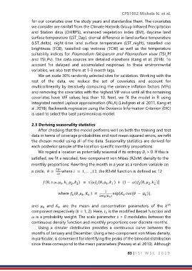
We regard a location as potentially seasonal if its entropy > 0. If this is
satisfied, we fit a rescaled, two-component von Mises (R2vM) density to the
monthly proportions. Rewriting the month in a year as a random variable on
2
a circle, = where = 1, … , 12, the R2vM function is defined as: 12
12
(, , , , ) = [ (, , ) + (1 − ) (, , )]
1
1
1
1
1 2
2
2
2
2

1
where (, , ) = exp{ ( − )},

2 0 ( )

and and are the mean and concentration parameters of the
ℎ

component respectively ( = 1, 2). Here, is the modified Bessel function and
0
is a probability weight. The scale parameter > 0 modulates between the
continuous density function and monthly proportions over discrete months.
Using a circular distribution provides a continuous curve between the
months of January and December. Using a two-component von Mises density,
in particular, is convenient for identifying the peaks of the bimodal distribution
since these correspond to the mean parameters (Pewsey et al. 2013). Although
83 | I S I W S C 2 0 1 9