Page 174 - Contributed Paper Session (CPS) - Volume 4

CPS2166 Divo Dharma Silalahi et al.
 l o ) l o 
  (v 2 x SSX  (v 2 x SSY )
m o g o comp; g o o g o comp; g o  (2)
=
VIP = o x  g o 1 + g o = 1 

ortho
2 SSX SSY
 cum cum 
 
 
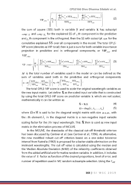
the sum of square ( SS ) both in variable y and variable X has subscript

comp g ; and comp ; g for the explained SS of g th component in the predictive
o
and g th component in the orthogonal, then the SS with subscript cum for the
o
cumulative explained SS over all components in the model. The total OPLS-
VIP score (denotes as VIP-total) then is just a sum for both variable importance

projection in predictive and in orthogonal components; or VIP pred and
VIP ortho
  l o 2 ) l 2 l o ( 2 ) l 2 ) (3)

M  g o =1 (  v o g o x SSX comp; g o g =1 (  v g x SSX comp; g )  v o g o x SSY comp; g o g =1 (  v g x SSY comp; g 
=1
VIP − total = x  + + g o + 
2  SSX cum SSX cum SSY cum SSY cum 
   
M is the total number of variables used in the model or can be defined as the
sum of variables used both in the predictive and orthogonal components
;
  
   SSX SSY    SSX cum; SSY cum;    .

 = M  cum g ; + cum g ;    m 0 = M  g o + g o  
m
    SSX cum SSY cum       SSX cum SSY cum   

The total OPLS-VIP score is used to scale the original wavelength variables as
~
the new input matrix. Let define X as the scaled input variable that is constructed
by using the total OPLS-VIP score on predictor variable X which are not scaled,
mathematically it can be written as
~
X = X Ω (4)
Ω = diag (λ , λ , λ , m ) (5)
2
1
where   is said to be the diagonal weight matrix with size m x m , with
Ω

the i th element λ in the diagonal matrix is a non-negative input variable
j
~
scaling factor for the j th input wavelength. This X then is used as new input
matrix in the elimination process of MCUVE.
In the MCUVE, the drawbacks of the classical cut-off threshold criterion
had been discussed by Centner et al. (see Centner et al., 1996). As alternative,
the new modified robust cut-off criterion based on a one-sided tolerance
interval from Natrella (1963) is proposed for a better stable elimination on the
irrelevant wavelengths. The cut-off value is calculated using the median and
the Median Absolute Deviation (MAD) of the reliability coefficients obtained
from the added artificial uninformative random variable. In addition, it includes
the value of k factor as function of the desired proportions, level of error, and

number of repetition used in MC random subsample selection. Using the c artif

163 | I S I W S C 2 0 1 9