Page 320 - Contributed Paper Session (CPS) - Volume 4

CPS2245 Azrie Tamjis
capture inefficiency. is assumed to be drawn from a half-normal
distribution with mean zero and variance . , can be estimated by using the
conditional mean of inefficiency term, given the composed error term, as
proposed by Jondrow et al. (1982) and derive the log-likelihood for
2
inefficiency, which is expressed in terms of the two variance parameters, =
2
2
+ capturing the variance of the composed error term = / , which
2
2
measures the fraction of inefficiency relative to statistical noise. Moreover,
can be used to measure the level of inefficiency of banks. For instance, if is
equal to 0, it indicates that there is no inefficiency based on the production
function imposed. On the other hand, if is more than 0, it indicates that
inefficiency is present. In the past, most studies using SFA were directed
towards inefficiency prediction and this inefficiency is commonly measured
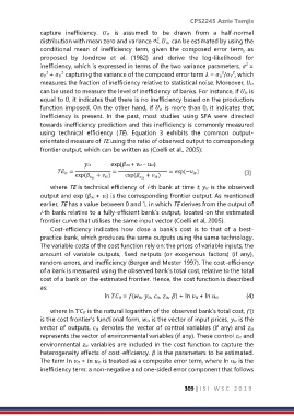
using technical efficiency (TE). Equation 3 exhibits the common output-
orientated measure of TE using the ratio of observed output to corresponding
frontier output, which can be written as (Coelli et al., 2005):

exp( + − )

where TE is technical efficiency of i-th bank at time t, is the observed
output and exp ( + ) is the corresponding frontier output. As mentioned
earlier, TE has a value between 0 and 1, in which TE derives from the output of
i-th bank relative to a fully-efficient bank’s output, located on the estimated
frontier curve that utilises the same input vector (Coelli et al, 2005).
Cost-efficiency indicates how close a bank’s cost is to that of a best-
practice bank, which produces the same outputs using the same technology.
The variable costs of the cost function rely on: the prices of variable inputs, the
amount of variable outputs, fixed netputs (or exogenous factors) (if any),
random errors, and inefficiency (Berger and Mester 1997). The cost-efficiency
of a bank is measured using the observed bank’s total cost, relative to the total
cost of a bank on the estimated frontier. Hence, the cost function is described
as:
ln = (, , , , ) + ln + ln (4)

where ln is the natural logarithm of the observed bank’s total cost, ()
is the cost frontier’s functional form, is the vector of input prices, is the
vector of outputs, denotes the vector of control variables (if any) and
represents the vector of environmental variables (if any). These control and
environmental variables are included in the cost function to capture the
heterogeneity effects of cost-efficiency. is the parameters to be estimated.
The term ln + is treated as a composite error term, where ln is the
inefficiency term: a non-negative and one-sided error component that follows

309 | I S I W S C 2 0 1 9