Page 146 - Contributed Paper Session (CPS) - Volume 5

CPS1159 Philip Hans Franses et al.
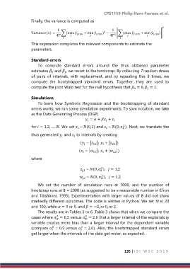
Finally, the variance is computed as

2
1 1
2
() = ∑(max ̂ + min ̂ ) − [∑(max ̂ + min ̂ )]
4 ,| ,| 4 2 ,| ,|

This expression completes the relevant components to estimate the
parameters.

Standard errors
To compute standard errors around the thus obtained parameter
̂
̂
estimates and , we resort to the bootstrap. By collecting T random draws
1
0
of pairs of intervals, with replacement, and by repeating this B times, we
compute the bootstrapped standard errors. Together, they are used to
compute the joint Wald test for the null hypothesis that = 0, = 1.
0
1

Simulations
To learn how Symbolic Regression and the bootstrapping of standard
errors works, we run some simulation experiments. To save notation, we take
as the Data Generating Process (DGP)
= + +

2
for = 1,2, … , . We set ~ (0,1) and ~ (0, ). Next, we translate the

thus generated and to intervals by creating

( − | |; + | |)

1,
2,

( − | |; + | |)
1,

2,
where

2
~ (0, ), = 1,2
,

2
~ (0, ), = 1,2
,

We set the number of simulation runs at 1000, and the number of
bootstrap runs at B = 2000 (as suggested to be a reasonable number in Efron
and Tibshirani, 1993). Experimentation with larger values of B did not show
markedly different outcomes. The code is written in Python. We set N at 20
and 100, while = 0 or 5, and = −2, or 0, or 2.
The results are in Tables 3 to 6. Table 3 shows that when we compare the
cases where = 0.5 versus = 2.0 that a larger interval of the explanatory
2
2

variable creates more bias than a larger interval for the dependent variable
2
2
(compare = 0.5 versus = 2.0). Also, the bootstrapped standard errors

get larger when the intervals of the data get wider, as expected.
135 | I S I W S C 2 0 1 9