Page 43 - Contributed Paper Session (CPS) - Volume 5

CPS795 Nestor B.
In our work denote the rainfall of day , indicates the dynamics of

rainfall on day , and be the state space of dynamics of rain-fall, for
example we can take = {1, 2} where the states 1 and 2 are favorables
respectively to wet days and dry days. The transition matrix of the Markov
chain ( ) is given by transition probabilities Pr( = | −1 = ) 1 ≤

≥0
, ≤ , which time dependent. To account for seasonality, logistic
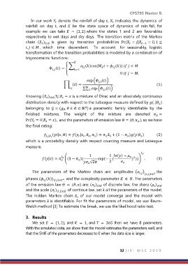
transformation of the transition probabilities is modeled by a combination of
trigonometric functions:

∑ ()cos ( + ()) <
Φ () = { =1
,
0 = .

exp ( ())
,
∏ () = . (1)
∑ exp ( ())
,
=1
Knowing ( ) | = is a mixture of Dirac and an absolutely continuous

≥0,
distribution density with respect to the Lebesgue measure defined by (. | )

belonging to = ( , ∈ ⊂ ℝ ) a parametric family identifiable by the

finished mixtures. The weight of the mixture are denoted =

Pr( = 0| = ), and the parameters of emission law Θ = (, ), so we have

the final rating:
| (|, Θ) = ( | , , ) = + (1 − )(| ) (2)

0

which is a probability density with respect counting measure and Lebesgue
measure.
1
1 1 ln() −
2
(|) = ((1 − )( exp (− ( ) ))) . (3)
0

√2 2

The parameters of the Markov chain are: amplitudes ( ) (.)∈ 2 the
,
2 and the complexity parameter ∈ . The parameters
phases ( ()) (,)∈ ,

of the emission law Θ = (, ) are: ( ) of discrete law, the sharp ( )
∈
∈
and the scale ( ) of continue law. set λ all the parameters of the model.
(.)∈
The hidden Markov chain of our model converge and the model with

parameters is identifiable. For fit the parameters of model, we use Baum-
Welch method [3] To estimate the break, we use the likelihood ratio test.

3. Results
We set = {1, 2}, and = 1, and = 365 then we have 8 parameters.
With the simulated data, we show that the model estimates the parameters well, and
that the SME of the parameters decreases to 0 when the data size is larger.
32 | I S I W S C 2 0 1 9