Page 61 - Contributed Paper Session (CPS) - Volume 5

CPS886 Marcelo Bourguignon
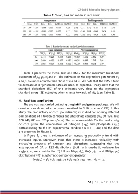
Table 1: Mean, bias and mean square error

Table 1 presents the mean, bias and RMSE for the maximum likelihood

estimators of 0, 1, 0 and 1. The estimates of the regression parameters 0
and 1 are more accurate than those of 0 and 1. We note that the RMSEs tend
to decrease as larger sample sizes are used, as expected. Finally, note that the
standard deviations (SD) of the estimates very close to the asymptotic
standard errors (SE) estimates when tends towards infinity (see, Table 2).

4. Real data application
The analysis was carried out using the glmBP and gamlss packages. We will
consider a randomized experiment described in Griffiths et al. (1993). In this
study, the productivity of corn (pounds/acre) is studied considering different
combinations of nitrogen contents and phosphate contents (40, 80, 120, 160,
200, 240, 280 and 320 pounds/acre). The response variable Y is the productivity
of corn given the combination of nitrogen ( ) and phosphate ( )
1
2
corresponding to the th experimental condition ( = 1, . . . ,30) and the data
are presented in Figure 1.
In Figure 1, there is evidence of an increasing productivity trend with
increased inputs. Moreover, note that there is increased variability with
increasing amounts of nitrogen and phosphate, suggesting that the
assumption of GA or RBS distributions (both with quadratic variance) for
log( ),i.e., we consider that follows BP( , ), GA( , ) and RBS( , )

distributions with a systematic component given by
log( ) = + log( ) + log( ) = 0.
0

1
2
2 2
1

50 | I S I W S C 2 0 1 9