Page 60 - Contributed Paper Session (CPS) - Volume 5

CPS886 Marcelo Bourguignon

∈ ℝ , with + < , 1 and 2 are the linear predictors, and =

T
( , . . . , ) and = ( , . . . , ) are observations on p and q known
T

1

1

regressors, for = 1, . . . , . Furthermore, we assume that the covariate matrices
T
T
= ( , . . . , ) and = ( , . . . , ) have rank p and q, respectively. The link
1

1
+
functions : ℝ → ℝ + and : ℝ → ℝ in (5) must be strictly monotone,
1
2
⊺
positive and at least twice differentiable, such that = 1 −1 ( )and =

⊺
2 −1 ( ), with −1 (∙) and 2 −1 (∙) being the inverse functions of (∙) and
1
1

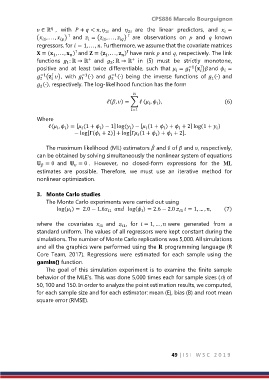
(∙), respectively. The log-likelihood function has the form
2

ℓ(, ) = ∑ ℓ ( , ), (6)

=1

Where
ℓ( , ) = [ (1 + ) − 1] log( ) − [ (1 + ) + + 2] log(1 + )

− log[Γ( + 2)] + log[Γ (1 + ) + + 2].

̂
The maximum likelihood (ML) estimators and ̂ of and , respectively,
can be obtained by solving simultaneously the nonlinear system of equations
= 0 and = 0 . However, no closed-form expressions for the ML

estimates are possible. Therefore, we must use an iterative method for
nonlinear optimization.

3. Monte Carlo studies
The Monte Carlo experiments were carried out using
log( ) = 2.0 − 1.6 log( ) = 2.6 − 2.0 = 1, … , , (7)

1
1

where the covariates 1 and , for = 1, … , were generated from a
1
standard uniform. The values of all regressors were kept constant during the
simulations. The number of Monte Carlo replications was 5,000. All simulations
and all the graphics were performed using the R programming language (R
Core Team, 2017). Regressions were estimated for each sample using the
gamlss() function.
The goal of this simulation experiment is to examine the finite sample
behavior of the MLE’s. This was done 5,000 times each for sample sizes (n) of
50, 100 and 150. In order to analyze the point estimation results, we computed,
for each sample size and for each estimator: mean (E), bias (B) and root mean
square error (RMSE).

49 | I S I W S C 2 0 1 9