Page 127 - Contributed Paper Session (CPS) - Volume 7

CPS2044 Mohd Asrul Affendi A. et al.
0, ℎ
= {

1, ℎ
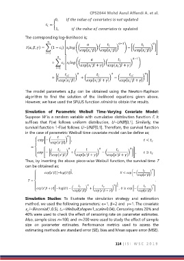
The corresponding log‐likelihood is;
−1

(, , ) = ∑(1 − ) [ (( [ ] ) ( [ ] ) ) − [( [ ] ) ]]

′
′
′
=1
−1

+ ∑ [ (( [ + ] ) ( [ + ] ) )

′
′
=1

+ [( ) + ( ) − ( ) ]]
′
′
[ ] [ + ] [ + ]
′

The model parameters a,β,γ can be obtained using the Newton‐Raphson
algorithm to find the solution of the likelihood equations given above.
However, we have used the SPLUS function nlminb to obtain the results.

Simulation of Parametric Weibull Time-Varying Covariate Model:
Suppose W is a random variable with cumulative distribution function F, it
suffices that F(w) follows uniform distribution, U~UNIF[0,1]. Similarly, the
survival function 1‐F(w) follows U~UNIF[0,1]. Therefore, the survival function
in the case of parametric Weibull time covariate model can be define as;

[− ( ) ] , <
′
[ ]
=

[− [( ′ ) + ( ′ ) − ( ′ ) ]] , ≥
{ [ ] [ + ] [ + ]
Thus, by inverting the above piece‐wise Weibull function, the survival time T
can be obtained as;
1
′
[ ][−log ()], < [− ( ′ ) ]
[ ]
= .
1

[ + ] [− log() − ( ) + ( ) ] , ≥ [− ( ) ]
′
′
′
′
{ [ ] [ + ] [ ]
Simulation Studies: To illustrate the simulation strategy and estimation
method, we used the following parameters; α=1, β=2 and γ=1. The covariate
x_i~Binomial(1,0.5), tci~Weibull(shape=1,scale=0.04). Censoring rates 20% and
40% were used to check the effect of censoring rate on parameter estimates.
Also, sample sizes n=100, and n=200 were used to study the effect of sample
size on parameter estimates. Performance metrics used to assess the
estimating methods are standard error (SE), bias and Mean square error (MSE).

114 | I S I W S C 2 0 1 9