Page 302 - Contributed Paper Session (CPS) - Volume 7

CPS2105 Hermansah et al.
2. Method
a. ARMA model
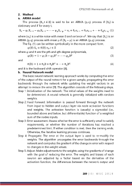
The process {X , t ∈ ℤ} is said to be an ARMA (p, q) process if {X } is
t
t
stationary and if for every t,

X − φ X − φ X − ⋯ − φ X = e + θ e + θ e + ⋯ + θ e (1)
t
1 t−1
1 t−1
2 t−2
2 t−2
p t−p
q t−q
t

where {e } is a white noise with mean 0 and variance σ . We say that {X } is an
2
t
t
ARMA (p, q) process with mean μ if {X − μ} is an ARMA (p, q) process.
t
The Eq. (1) can be written symbolically in the more compact form,
φ(B) X = θ(B) e , t ∈ ℤ (2)
t
t
where φ and θ are the pth and qth degree polynomials,
φ(B) = 1 − φ B − φ B − ⋯ − φ B (3)
p
2
1
p
2
and
2
q
θ(B) = 1 + θ B + θ B + ⋯ + θ B (4)
q
2
1
and B is the backward shift operator [8].
b. Neural Network model
The basic neural network learning approach works by computing the error
of the output of the neural network for a given sample, propagating the error
backwards through the network while updating the weight vectors in an
attempt to reduce the error [9]. The algorithm consists of the following steps.
Step 1: Initialization of the network: The initial values of the weights need to
be determined. A neural network is generally initialized with random
weights.
Step 2: Feed Forward: Information is passed forward through the network
from input to hidden and output layer via node activation functions
and weights. The activation function is (usually) a sigmoidal (i.e.,
bounded above and below, but differentiable) function of a weighted
sum of the nodes inputs.
Step 3: Error assessment: Assess whether the error is sufficiently small to satisfy
requirements, or whether the number of iterations has reached a
predetermined limit. If either condition is met, then the training ends.
Otherwise, the iterative learning process continues.
Step 4: Propagate: The error at the output layer is used to re-modify the
weights. The algorithm propagates the error backwards through the
network and computes the gradient of the change in error with respect
to changes in the weight values.
Step 5: Adjust: Make adjustments to the weights using the gradients of change
with the goal of reducing the error. The weights and biases of each
neuron are adjusted by a factor based on the derivative of the
activation function, the differences between the network output and

289 | I S I W S C 2 0 1 9