Page 95 - Contributed Paper Session (CPS) - Volume 8

CPS2204 T. von R. et al.
(, ) = (( , ), … , ( , )) = ( (), … , ()) .

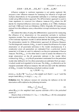
1
1

Influence analysis in nonlinear regression is not widely explored. We
propose a new influence measure for assessing the influence of single and
multiple observations on the parameter estimates in a nonlinear regression
model using differentiation approach. The differentiation approach is used in
linear regression to construct the influence measure ̂ where the EIC
,
stands for Empirical Influence Curve (see e.g. Belsley et al. (1980), Chatterjee
and Hadi (1988) and Cook and Weisberg (1982)). Originally EIC measure was
derived from the influence curve, a theoretical concept introduced by Hampel
(1974).
We extend the ideas of using the differentiation approach for measuring
the influence of an observation on the parameter estimate in nonlinear
regression models. Two new influence measures for the parameter estimates
in the nonlinear regression model (1) will be derived: the ̂ and ̂ , .

,
The abbreviation stands for Differentiation approach & Influence Measure.
The first diagnostic measure, ̂ , is used to assess the influence of a single
,
observation on all parameter estimates in the model, simultaneously. It is
constructed when all parameters are estimated from a perturbed model,
presented in (2) later on, and it is referred to as the joint-parameter influence
measure. The ̂ , ., on the other hand, is used to assess the influence of a

single observation on the jth parameter estimate in the model. When
constructing ̂ , ., only the jth parameter is estimated from the perturbed

model, later defined in (2): the other parameters are estimated from an unper-

b turbed model and regarded to be known. The ̂ is referred to as the
,,
marginal-parameter influence measure. We will now start with the definition
of ̂ . Consider the following perturbed nonlinear model
,
= (, ) + , (2)

−1
2
where ~ (, ( )), is the weight such that 0 < ωk ≤ 1 and the

weight matrix ( ) = (1, … . , , …,1).

Definition 2.1. The influence measure for assessing the influence of the kth
̂
observation on is defined as the following derivative

̂ = ( )| =1, (3)
,

̂
where ( )is the weighted least squares estimate of in the perturbed

model (2).
̂
̂
Observe that, in Definition 2.1, if ωk → 1, then ( ) → , the unweighted

least squares estimate.
84 | I S I W S C 2 0 1 9