Page 96 - Contributed Paper Session (CPS) - Volume 8

CPS2204 T. von R. et al.
To calculate the ̂ in (3) we need an estimator for in the perturbed
,
model (2). Using the method of weighted least squares, which is equivalent to
the maximum likelihood approach, we have to find ̂ that minimizes the
following

( ) = ( − (, )) ( )( − (, ))

Differentiating Q(ωk) with respect to and solving normal equations using
iterative methods (e.g. the GaussNewton method), the obtained least squares
estimate of is obtained as a function of ωk. In the next theorem, the explicit
expression of ̂ , defined in (3), is presented.
,
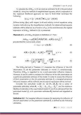
Theorem 2.1. Let ̂ be given in Definition 2.1. Then
,
−
̂

̂
̂
̂
̂ = () ((() () − ()( ⊗ )) ,

,

provided that the inverse exists, where
̂
= ( ) = − (, ), (4)

(, )
̂
̂
̂
() = ( (), … , ()) = | , × . (5)

1

= ̂
and
̂
(, ) ()
̂
() = ( ( )) = , × (6)
̂

= ̂

The ̂ derived in Theorem 2.1 measures the influence of the th
,
observation on all the parameter estimates in model (1) simultaneously.
Therefore, ̂ is regarded to be a joint-parameter influence measure.
,
However, it can be useful to measure the influence of the th observation on
a particular parameter estimate of the model. In order to assess the influence
̂
of the k observation on the th parameter estimate, , a marginal-parameter

influence measure will be defined, and its explicit expression will be derived.
̂
̂ ̂
Consider the perturbed model (2). Let = ( , ) be a vector of

1
̂
̂
̂
̂

parameter estimates, where = ( , … , −1 , ̂ +1 , … ) , are the maximum
1

1
̂
likelihood estimates in the unperturbed model (1) and is estimated from the

̂
perturbed model (2), with parameter estimates inserted and regarded as
1
known.

Definition 2.2. The marginal influence measure for assessing the influence of
̂
the th observation on the parameter estimate is defined as the following

derivative.
85 | I S I W S C 2 0 1 9