Page 339 - Contributed Paper Session (CPS) - Volume 6

CPS1950 Paolo G. et al.
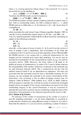
where  is a tuning parameter taking values in the interval [0, 1]. It can be
shown that (5) can be rewritten as
fFRFKM = || X[AA + (1) (IAA)]  UFA || . (6)
2
1/2
Therefore, the FRFKM model can be formulated as
1/2
X[AA + (1) (IAA)] = UFA + E. (7)
The FRFKM procedure contains several clustering methods as special case. In
fact, if U is a membership matrix, the FKM is obtained when  = 1, whilst
FRFKM reduces to RKM when  = 0. Furthermore, if Q = J, A = IJ and thus (7)
is simplified as
X= UF + E, (8)
which resembles the well-known Fuzzy K-Means algorithm (Bezdek, 1981) in
case U is a fuzzy membership degree matrix (i.e., U  0I × K, and U1K = 1I).
Thus, the optimal parameter matrices U, F and A are found by minimizing (6)
subject to the following constraints:
U  0I × K, (9)
U1K = 1I, (10)
AA = IQ, (11)
where 0I × K is the matrix of zeroes of order (I × K), 1K and 1I are the vectors of
ones of lengths K and I, respectively. The minimization of (6) under the
constraints in (9)-(11) can be done by an ALS algorithm. As for FKM and RKM,
the FRFKM solution is not unique due to rotational indeterminacy for the
weights and the centroids and cluster label switching. This can be used to
simplify the interpretation of the components by means of, e.g., the varimax
procedure (Kaiser, 1958). Moreover, the fuzzy nature of U leads to an
additional source of indeterminacy. In order to fix it and to further improve
the interpretability of the solution, additional constraints on the centroids may
be used following Suleman (2015). This is motivated by the fact that the
optimal centroid matrix F can be determined by regression. This does not
guarantee that the estimated centroids have a reasonable meaning. For this
purpose, we can constrain the centroids to be convex combinations of the
observation units according to the so-called archetypal analysis (see, for
instance, Cutler & Breiman, 1994; Epifanio et al., 2018). In detail, Suleman
(2015) proposes to estimate the centroids by means of a particular archetypal
analysis where the weights of the convex combinations are equal to the fuzzy
membership degrees. In the current framework, it may be convenient to
estimate the centroids in a similar way by considering a weighted mean of the
observation units projected on the subspace spanned by the columns of A.
2.4.1. Choice of Q, K and :
The selection of the number of components Q, the number of clusters K
and the weighting parameter  can be done subjectively or according to
model selection heuristics by using different triplets of values for Q, K and .
Note that the selection of  can be done by considering a subset of values in

328 | I S I W S C 2 0 1 9