Page 361 - Contributed Paper Session (CPS) - Volume 6

CPS1966 Jessa L. S. C. et al.
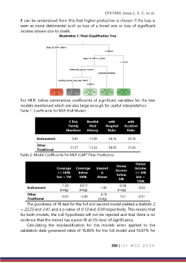
It can be understood from this that higher protection is chosen if the loss is
seen as more detrimental such as loss of a loved one or loss of significant
income stream due to death.
Illustration 1: Final Classification Tree

For MLR, below summarizes coefficients of significant variables for the two
models mentioned which are also large enough for useful interpretation.
Table 1: Coefficients for MLR (Full Model)

3 Sick NonStd with with
Family Med Hospital Accident
Members History Rider Rider

Endowment 0.81 -12.09 -14.76 20.76

Other -17.27 -15.53 -18.95 21.56
Traditional
Table 2: Model Coefficients for MLR (CART Final Predictors)

Owner Owner
Coverage Coverage Insured Income Income
=> 500k below is => 50k
but < 1M 500k Owner below but <
50k
150K
-1.30 0.017 -0.38
Endowment -1.85 -0.65
(insig) (insig) (insig)
Other -3.61 -3.00 0.79 1.61 -0.31
Traditional (insig)
The goodness-of-fit test for the full and second model yielded a statistic C
= 22.25 and 3.41, and a p-value of 0.13 and 0.99 respectively. This means that
for both models, the null hypothesis will not be rejected and that there is no
evidence that the model has a poor fit at 5% level of significance.
Calculating the misclassification for the models when applied to the
validation data generated rates of 16.85% for the full model and 16.07% for

350 | I S I W S C 2 0 1 9