Page 359 - Contributed Paper Session (CPS) - Volume 6

CPS1966 Jessa L. S. C. et al.
chosen for each method. These are 70%-30% or 4 folds for CART, 50%-50%
for MLR, and 80%-20% for full model Random Forest and 50%-50% for
Random Forest with CART variables which will be explained later.
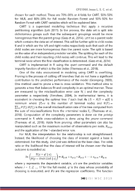
CART is a supervised modelling technique that apply a recursive
partitioning algorithm (Loh 2011). In the process, the data set is split into
dichotomous groups such that the subsequent groupings would be more
homogenous than the parent group (Gass et al., 2014). Let t be a parent node
which contains the data set of interest. This will be further split to child nodes
tl and tr which are the left and right nodes respectively such that each of the
child nodes are more homogenous than the parent node. The split is based
on the value of an independent predictor variable. The splitting for each of the
child nodes and their resulting child nodes will continue. This will lead to the
terminal node where the final classification is determined. (Gass et al., 2014)
CART is implemented in R using the rpart command and the default
impurity function of which is the Gini Index (Therneau et al., 2018).
One of the risks encountered in modeling using CART is overfitting.
Pruning is the process of cutting off branches that do not have a significant
contribution to the predictive performance of the model (Gromping. 2009),
One method used to prune a tree is cross-validation. This method aims to
generate a tree that balances fit and complexity in an optimal manner. These
are measured by the misclassification error cate R( ) and the complexity
parameter α respectively (Timofeev, 2004), In mathematical terms, it is
equivalent in choosing the optimal tree T such that Rα (T) = R(T) + α|T| is
minimum where |T|=v is the number of terminal nodes and () =
∑ ( ) ( ) is the overall misclassification rate of the tree computed from

=1
the sum of misclassifications from the v terminal nodes , (Therneau et al.,

2018). Computation of the complexity parameters is done via the printcp
command in R while cross-validation is done using the prune command
(Themeau et al., 2018). Aside from pruning. other parameters can also be
manipulated such as the maximum number of observations per node, ,
and the application of the 1-standard error rule.
For MLR, the interpretation for the relationship is not straightforward.
Instead, the likelihood of choosing the class of interest against a base is
determined. For this study, Unit Link was defined as the base class. The odds
ratio or the likelihood that the class of interest will be chosen over the base
outcome is modelled as:

where y represents the dependent variable, xi’s are the predictor variables
where i = 1, 2, …, 17 for the full model, q’ is the class whose probability of
choosing is evaluated, and B’s are the regression coefficients. The function

348 | I S I W S C 2 0 1 9