Page 397 - Contributed Paper Session (CPS) - Volume 6

CPS1995 Daniel B. et al.
̂
If is the MLE, its limiting distribution can be used to draw inferences on
̂
′
, = 1, … , . Using the fact that → (, −1 ()), where () = −(())
′
−1/2
̂
The standard error of the estimator , of , is given by ′ () where ()

′

is the i’th diagonal element of () [see Serfling, R.J. (1980)]. Thus, an
1
−
̂
2 ̂
approximate 95% confidence interval for is given by , ±1.96 ( , ). A

′
′
test for the general hypothesis : = can be conducted based on a Wald-
0
̂
̂
′
2
2
type statistic = ( − )′( −1 () )′( − ) . Under H, 2 → ,

0

0
where = ().
To simplify model construction, we assume that F belongs to the family of
exponential distributions, i.e., the probability density (mass) function is given

by (; ) = ℎ(){∑ ′ () () − ()}. The exponential family is said
′
′
=1
′
to be in canonical form if () = , = 1, … , and it said to be curved if
′
′
dim(Θ) < dim((Θ)). In the simplest case, i.e., canonical representation with r
= 1, we assume that () = ′ , where = (|, ), z is the vector of
covariates (fixed and random), is the vector of structural parameters and
(. ) is the link function. This defines a generalized linear model representation
for Y.

3. Result
We now provide some constructions for extrapolation under a generalized
linear mixed model setting using interval information. These constructions can
certainly be extended to allow for more involved extrapolation cases.
a. Extrapolation with Normal Latent Variables
We consider the simple case where ( ) = + + + .
1 1
0

3 3
2 2
In this representation, 1 , for all = 1, … , , is the fixed subject covariate
where = 1, … , represents the subjects associated with p different

estimands. Furthermore, is the fixed estimand covariate where = 1, … , .
2
Lastly, 3 represents the treatment covariate. Also, we assume that the latent
variable Y is normally distributed and observed in terms of the ordinal variable
̃
through the intervals ( −1, , ], = 1, … , as defined in Section 2. Note
,
that in applications, the fixed covariates for subject and estimand are
measured through proxy variables to facilitate the estimation of the fixed
subject effect 1 and fixed estimand effect 2.
′
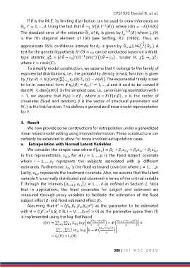
Assuming that = ( , , , ) as the parameter to be estimated
2
1
0
3,
2
with Θ = {( , ): ∈ ℝ, = 0, … ,3; > 0} as the parameter space then (1)
2
′
2

is implemented using the log-likelihood

386 | I S I W S C 2 0 1 9