Page 398 - Contributed Paper Session (CPS) - Volume 6

CPS1995 Daniel B. et al.
′
Where ( , … , −1 ) represent the right-censored counts and =
1

(1, 1 , , 3 ) are the covariates. Estimation of and testing of : = 0
2
will proceed as described in Section 2.
b. Extrapolation for Poisson Counts
Here we introduce a construction for modelling of event counts. We
assume that the underlying count process is a homogeneous Poisson process
with the conditional mean given by ( ) = log( ) = + log 1 +

0
log 2 + . In this representation, 1 is the random subject effect, whereas
1 3
2 is the random estimand effect. In a variety of applications, it is reasonable
to assume that 1=1112 where 11 represents the subject’s time at risk and 12
denotes frailty. For simplicity, one can assume that 11,12 and 2 are
independent and as in the previous construction we let 3j denote the
treatment covariate. Also, we assume that the latent homogeneous count
process Y is Poisson distributed and observed in terms of the ordinal variable
̃
through the integer intervals ( −1, , ], i = 1, … , k as defined in Section 2.
,
′
′
Conditional on = 1 and = and assuming that = ( , , )
2
2
1
1
0
′
′
as the parameter to be estimated with Θ = {( , ): ∈ ℝ, = 0,1; ∈

ℝ } as the parameter space and denoting the vector of nuisance parameters
associated with time at risk, frailty, and estimand effect, then (1) can be
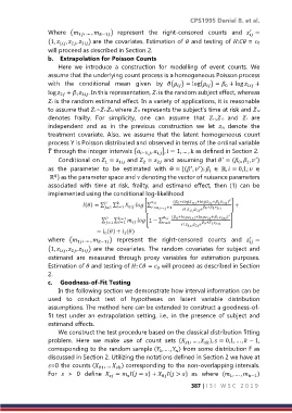
implemented using the conditional log-likelihood

′
where ( , … , −1 ) represent the right-censored counts and =

1
(1, 1 , , 3 ) are the covariates. The random covariates for subject and
2
estimand are measured through proxy variables for estimation purposes.
Estimation of and testing of : = will proceed as described in Section
0
2.
c. Goodness-of-Fit Testing
In the following section we demonstrate how interval information can be
used to conduct test of hypotheses on latent variable distribution
assumptions. The method here can be extended to construct a goodness-of-
fit test under an extrapolation setting, i.e., in the presence of subject and
estimand effects.
We construct the test procedure based on the classical distribution fitting
problem. Here we make use of count sets ( , … , ), = 0,1, … , − 1,

1
corresponding to the random sample ( , … , ) from some distribution F as
1

discussed in Section 2. Utilizing the notations defined in Section 2 we have at
=0 the counts ( , … ) corresponding to the non-overlapping intervals.

01
For > 0 define = { = } + { > } as where ( , … , −1 )

1
0
387 | I S I W S C 2 0 1 9