Page 144 - Invited Paper Session (IPS) - Volume 2

IPS192 Hukum C. et al.
the rows of X, Z and I that correspond to area . When is negligible
m

compared to , the SNLEP (9) is ̂ = ̂ . An estimate of the

proportion or rate in area is ̂ . In the spirit of Chandra et al. (2017) and
Opsomer et al. (2008), we develop a bootstrap procedure to test the spatial
2
nonlinearity hypothesis, that is, the hypothesis 2: = 0 versus the one-
0
2
sided alternative 2: > 0.
1

3. Empirical Evaluations
This Section presents the results from simulation studies that compare the
empirical performance of the proposed SNLEP estimator (9) under the
SNLGLMM (4) with the EP (3) under the GLMM (1). The performance criteria
used are the percentage Relative Bias (RB) and the percentage Relative Root
MSE (RRMSE). In our model based simulations we set the number of small
areas = 100 and considered two values for the area specific sample sizes
=10 and 50 with = 100 and 5000, respectively.

We used an area level version GLMM to generate data. The response
values were generated from ~Binomial ( , ) and logit( ) = ƞ = ( ) +

with = exp(ƞ ){1 + exp (ƞ } −1 . Spatial locations were simulated as the

values of two independently distributed uniform [0,1] covariates and ,
1
2
and the random area effects were generated as independent realizations

2
from a (0, = 0.0625) distribution. We considered two different choices of

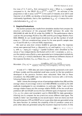
the response function ( , ): Plane ( , ) = 0.5 + 0.2 ,
2
2
1
2
1
1

2
2
40 exp[8{( 1 −0.5) + ( 2 −0.5) }]
Mountain : ( , ) = exp[8{( 1 −0.2) +( 2 −0.7) }]+exp[8{( 1 −0.7) +( 2 −0.2) }]
1
2
2
2
2
2

A total of = 1000 data sets were independently generated under each
of these models and the predicted small area counts for the two predictors
developed in the previous Sections were calculated. Note that in these
simulations the SNLGLMM uses the radial basis functions with =25 knots,
following Pratesi et al. (2009).
Table 1 shows the average values of percentage relative bias (RB) and the
average values of percentage relative root MSE (RRMSE) recorded by the SAE
methods investigated in our simulations. In particular, Table 1 sets out the
average relative biases and the average relative RMSEs of the two small area
predictors (EP and SNLEP) across the two different types of response function
( , ) (i.e. plane and mountain) used in SNLGLMM for data generation,
2
1
allowing one to compare the two predictors across different data types. The
results in Table 1 are essentially as one would expect. Here we clearly see that
the performances of EP and SNLEP are on a par when data are generated using
the plane function. In contrast, the simplicity of the EP predictor comes at a
price when data are generated using the mountain response function. In this
131 | I S I W S C 2 0 1 9