Page 364 - Invited Paper Session (IPS) - Volume 2

IPS279 Rense Lange
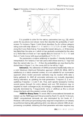
Figure 1: Probability of Observing Ratings w= 0, 1, and 2 as Respondents’ Trait Levels
(T) Increase.

It is possible to solve for the various parameters (see e.g., [3]), which
yields the equations (not shown here) that describe the probability of each
answer. For instance, Figure 1 (solid lines) describes Pijkw for a three-category
rating scale with step values F1 = -1.1 and F2 = 1.1, S = D = 0, with T varying
along the X-axis. Note that as T increases the lowest rating (i.e., w=0) becomes
less likely than the value w=1, which is then gradually superseded by the value
w=2. Note that w=0 and w=1 are equally likely to occur at T = F1 = -1.1 and
that w=1 and 2 occur with equal probability at T = F2 = 1.1.
The parameters combine additively in Equation 1, thereby facilitating
interpretation. For instance, if we had used a rater whose severity is 1 logit less
than the current rater (i.e., S = -1) then the probabilities are described by the
dotted lines in Figure 1, i.e., the curves shift to the left by 1 logit.
Estimation. The estimation of MFRS parameters traditionally relies on
a Joint Maximum Likelihood Estimation approach (JMLE) [2]. While JMLE is
satisfactory in a batch-oriented context, it is not suitable for an incremental
approach where model parameter estimates may be needed while data is
being gathered. In JMLE all parameter estimates are mutually dependent
during estimation, as updating the trait parameters T requires D, S, and F,
updating D requires T, S, and F, etc. Thus, each update necessarily involves
several passes through the entire dataset and over 200 iterations may be
required to reach convergence [4]. Accordingly, computational demands are
typically dominated by T (respondents’ traits or abilities) as this is almost
always the facet with the greatest number of levels.
PAIRS for Binary Items. To avoid JMLE’s computational demands we
instead use the PAIRS approach first proposed by Rasch [7], see [8]. To be sure,
PAIRS’ computational demands are also dominated by the levels of T.
However, with some pre-processing many required computations can already
be performed during data gathering while new data are entered. With all pre-
processing completed, obtaining the final parameter estimates requires very

351 | I S I W S C 2 0 1 9