Page 395 - Special Topic Session (STS) - Volume 3

STS551 Stephen Wu et al.
Data Set 1) All uncertainties are moved to the measurement error, i.e., = 0

and = 0.4. Each data point among the 1000 is generated

independently from a random measurement noise.
Data Set 2a) Each data point among the 1000 is generated independently
from a random noise for = 0.2 and a random noise for = 0.2.

Data Set 2b) For each data set , one fixed value of () is generated based

on = 0.2 and it is used to generate the 50 data points with

independent random noise for y = 0.2.

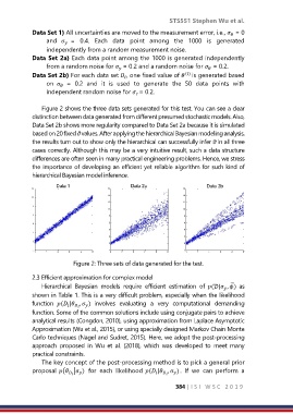
Figure 2 shows the three data sets generated for this test. You can see a clear
distinction between data generated from different presumed stochastic models. Also,
Data Set 2b shows more regularity compared to Data Set 2a because it is simulated
based on 20 fixed θ values. After applying the hierarchical Bayesian modeling analysis,
the results turn out to show only the hierarchical can successfully infer θ in all three
cases correctly. Although this may be a very intuitive result, such a data structure
differences are often seen in many practical engineering problems. Hence, we stress
the importance of developing an efficient yet reliable algorithm for such kind of
hierarchical Bayesian model inference.

Figure 2: Three sets of data generated for the test.

2.3 Efficient approximation for complex model
Hierarchical Bayesian models require efficient estimation of (| , ) as
⃗⃗

shown in Table 1. This is a very difficult problem, especially when the likelihood
function ( | , ) involves evaluating a very computational demanding

function. Some of the common solutions include using conjugate pairs to achieve
analytical results (Congdon, 2010), using approximation from Laplace Asymptotic
Approximation (Wu et al., 2015), or using specially designed Markov Chain Monte
Carlo techniques (Nagel and Sudret, 2015). Here, we adopt the post-processing
approach proposed in Wu et al. (2018), which was developed to meet many
practical constraints.
The key concept of the post-processing method is to pick a general prior
proposal ( | ) for each likelihood ( | , ). If we can perform a

384 | I S I W S C 2 0 1 9