Page 453 - Special Topic Session (STS) - Volume 3

STS555 Mohamed Salem Ahmed et al.
and

where , the limit of the sequence , is a nonrandom positive definite

matrix. The functions (∙,∙) and (∙,∙) are viewed as empirical counterparts

of (∙,∙) and (∙,∙) respectively. It is clear that (∙) is not available in practice.
0
However, we need to estimate it, particularly by an asymptotically efficient

estimate. By (5) and for fixed = ( , ) ∈ Θ an estimator of () for z ∈ Z

0
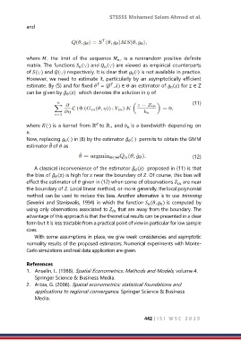
can be given by ̂ () which denotes the solution in of

(11)

where (∙) is a kernel from ℝ to ℝ and is a bandwidth depending on

+

.
Now, replacing (∙) in (8) by the estimator ̂ (∙) permits to obtain the GMM
0

estimator of as
̂
(12)
A classical inconvenience of the estimator ̂ () proposed in (11) is that

the bias of ̂ () is high for near the boundary of . Of course, this bias will

effect the estimator of given in (12) when some of observations are near

the boundary of . Local linear method, or more generally, the local polynomial
method can be used to reduce this bias. Another alternative is to use trimming
(Severini and Staniswalis, 1994) in which the function (, ) is computed by
0

using only observations associated to that are away from the boundary. The

advantage of this approach is that the theoretical results can be presented in a clear
form but it is less tractable from a practical point of view in particular for low sample
sizes.
With some assumptions in place, we give weak consistencies and asymptotic
normality results of the proposed estimators. Numerical experiments with Monte-
Carlo simulations and real data application are given.

References
1. Anselin, L. (1988). Spatial Econometrics: Methods and Models, volume 4.
Springer Science & Business Media.
2. Arbia, G. (2006). Spatial econometrics: statistical foundations and
applications to regional convergence. Springer Science & Business
Media.

442 | I S I W S C 2 0 1 9