Page 452 - Special Topic Session (STS) - Volume 3

STS555 Mohamed Salem Ahmed et al.

For simplicity of notation, we write when it is possible = ( , ) ∈ Θ =
Θ × Θ .

Note that in (6), the generalized residual (∙ ,∙) is calculated by
̃

conditioning only on not on the entire sample { , = 1,2, … , , =

1, … } or a subset of it. This of course will influence the efficiency of the
estimators of obtained by these generalized residuals, but it allows to avoid
a complex computation. To address this loss of efficiency, let us follow Pinkse
and Slade (1998)’s procedure that consists of employing some instrumentals
variables in order to create some moments conditions, and use some random
matrix to define a criterion function. Both the instrumentals variables and the
random matrix permit to take into account more informations about the
spatial dependence and heteroscedasticity in the dataset. Let us now detail
the estimation procedure.
Let

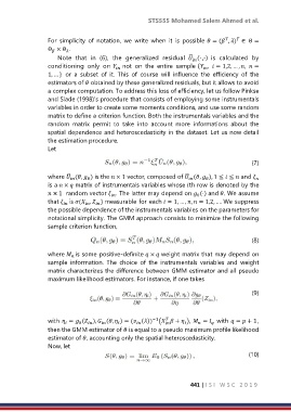
(7)

̃ ̃
where (, ) is the × 1 vector, composed of (, ), 1 ≤ ≤ and

is a × matrix of instrumentals variables whose th row is denoted by the
× 1 random vector . The latter may depend on (∙) and . We assume

0
that is ( , ) measurable for each = 1, … , , = 1,2, …. We suppress

the possible dependence of the instrumentals variables on the parameters for
notational simplicity. The GMM approach consists to minimize the following
sample criterion function,
(8)
where is some positive-definite × weight matrix that may depend on

sample information. The choice of the instrumentals variables and weight
matrix characterizes the difference between GMM estimator and all pseudo
maximum likelihood estimators. For instance, if one takes

(9)

with = ( ), (, ) = ( ()) ( + ), = with = + 1,

−1

0

then the GMM estimator of is equal to a pseudo maximum profile likelihood
estimator of , accounting only the spatial heteroscedasticity.
Now, let
(10)
441 | I S I W S C 2 0 1 9