Page 380 - Contributed Paper Session (CPS) - Volume 2

CPS1889 Subanar
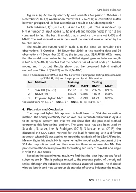
Figure 4: (a) An hourly electricity load Jawa-Bali for period 1 October -1
December 2016; (b) wcorrelation matrix for L = 672; (c) w-correlation matrix
between groups;and (d) four subseries as a result of SSA decomposition
()
Each subseries, {for = 1, … ,4 and = 1,2, … , − 24}, is modeled by

NN. A number of input nodes (6, 12, and 24) and hidden nodes (1 to 10) are
combined to find the best fit model, that is produce the smallest RMSE and
MAPE. The final forecast value is the sum of the forecast value obtained by the
four NN model.
The results are summarized in Table 1. In this case, we consider 1464
observations (1 October – 30 November 2016) as the training data and 24
observations (1 December 2016) as the testing data. SSALRF(86, 672) means
that the model is reconstructed by the 86 first eigentriples and window length
is 672. NN(24-10-1) denotes that the network has 24 input nodes, 10 hidden
nodes, and 1 output. Results show that the proposed hybrid method
outperforms SSA-LRF(86,672) and NN(24-10-1).

Table 1: Comparison of RMSEs and MAPEs for the training and testing data obtained
by SSA-LRF, NN, and the proposed hybrid NN method
No Method Training Testing
RMSE MAPE RMSE MAPE
1 SSA-LRF(86,672) 153.02 0.57% 236.78 0.96%
2 NN(24-10-1) 137.09 0.50% 116.15 0.41%
3 Proposed hybrid NN* 76.24 0.29% 64.29 0.24%
*obtained from NN(24-9-1)+NN(24-9-1)+NN(24-10-1)+NN(24-10-1)

4. Discussion and Conclusion
The proposed hybrid NN approach is built based on SSA decomposition
method. The hourly electricity load of Jawa-Bali is considered in this study due
to its complex pattern and thus we can show that the proposed method
overcomes this forecasting problem. The same data has also been used by
Sulandari, Subanar, Lee, & Rodrigues (2019). Sulandari et al. (2019) also
discussed the SSA-based method for the load forecasting with a different
approach where NN was applied to model the residuals of the SSA-LRF model.
Meanwhile, in this study, NN is implemented to model each component of the
SSA decomposition result and then combine them as an ensemble NN. This
proposed method can improve the forecasting accuracy of SSA-LRF and single
NN for the load series.
Based on the experimental result, we find that the best input nodes for all
subseries are 24. This is perhaps related to the seasonal period of the original
series, although the subseries does not show a seasonal pattern. The choice of
window length and how we group eigentriples of course influence the results.

369 | I S I W S C 2 0 1 9