Page 425 - Contributed Paper Session (CPS) - Volume 2

CPS1915 Han G. et al.
where denotes an input feature vector, and , and , denote the

maximum and minimum in the input vector, respectively.
ℎ

3. Result
The experiments were all performed using Python 3.7 and Sklearn library,
which relies on Numpy, Scipy, and matplotlib, and conducted in a Linux server
with an Intel Core i7 2.2 GHz processor. The neural network models for the
bank telemarketing data included one input layer with 20 input features and
output layer with one node. The optimal size of the hidden layer was
determined by tuning the number of nodes. The number of choice ranges
from 0 to 50. The number of iteration was set to be 10000 for all experiments.
The initial value of the learning rate is 1.2. Due to the limited space, the table
for the prediction accuracy values failed to show in the text which is available
from the corresponding author.
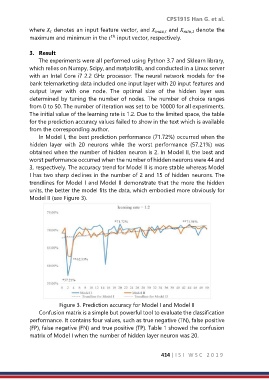
In Model I, the best prediction performance (71.72%) occurred when the
hidden layer with 20 neurons while the worst performance (57.21%) was
obtained when the number of hidden neuron is 2. In Model II, the best and
worst performance occurred when the number of hidden neurons were 44 and
3, respectively. The accuracy trend for Model II is more stable whereas Model
I has two sharp declines in the number of 2 and 15 of hidden neurons. The
trendlines for Model I and Model II demonstrate that the more the hidden
units, the better the model fits the data, which embodied more obviously for
Model II (see Figure 3).

Figure 3. Prediction accuracy for Model I and Model II
Confusion matrix is a simple but powerful tool to evaluate the classification
performance. It contains four values, such as true negative (TN), false positive
(FP), false negative (FN) and true positive (TP). Table 1 showed the confusion
matrix of Model I when the number of hidden layer neuron was 20.

414 | I S I W S C 2 0 1 9