Page 15 - Contributed Paper Session (CPS) - Volume 3

CPS1923 Deemat C M. et al.
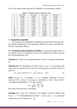
The critical values of the exact test for different are tabulated in Table 1.

Table 1. Critical values of the exact test
90% level 95% level 97.5% level 99% level
2 0.4000 0.4500 0.4750 0.4900
3 0.2764 0.3419 0.3883 0.4292
4 0.2189 0.2678 0.323 0.3693
5 0.1883 0.2383 0.28 0.325
6 0.1679 0.2131 0.2508 0.2927
8 0.1413 0.1799 0.2125 0.2492
10 0.1243 0.1586 0.1877 0.2208
20 0.0852 0.109 0.1295 0.1531
30 0.0689 0.0882 0.1049 0.1241
50 0.0529 0.0679 0.0808 0.0957
100 0.0373 0.0477 0.0569 0.0675

3. Asymptotic properties
In this section, we investigate the asymptotic properties of the proposed
test statistic. Making use of the asymptotic distribution we also calculate the
Pitman’s asymptotic efficacy.

3.1. Consistency and asymptotic normality. As the proposed test statistic is
a U-statistic, we use the asymptotic theory of U-statistics (Lee, 1990) to discuss
the limiting behaviour of ∆ .
̂ ∗

Theorem 3.1. The ∆ is a consistent estimator of ∆ ( ) under the alternatives
̂ ∗
∗
∗
.
1

Theorem 3.2. The distribution of √(∆ − ∆( )), as → ∞, is Gaussian with
̂
∗
mean zero and variance 4 , where is the asymptotic variance of ∆ and is
2
2
̂
1
1
given by
1
1
̅
∗
∗
∗ ∗
2
∗
= (2 ( ) + 2 ∫ 0 ∗ () − ) (2)
1
4
2

Proof: Since ∆ is a U-statistic it is a consistent estimator of ∆( )
∗
̂
(Lehmann,1951). Hence ∆ converges in probability to ∆( ). Note that
̅
̂
∗
∗
converges in probability to . As we can write
∗
∗
̂
∆ ∆( ) ∗
̂ ∗
∆ = . . ,
∗
̅ ∗
∆( ) ∗
the proof of the theorem is immediate.

Corollary 3.1. Let be continuous non-negative random variable with
∗

∗
∗
̅
∗
̂ ∗
() = − , then the distribution of √(∆ − ∆ ( )), as → ∞, is Gaussian
2
with mean zero and variance = 2 .
0
12
4 | I S I W S C 2 0 1 9