Page 16 - Contributed Paper Session (CPS) - Volume 3

CPS1923 Deemat C M. et al.
Corollary 3.2. Let be continuous non-negative random variable with
∗

−
() = then the distribution of √(∆ − ∆ ( )), as → ∞, is Gaussian
̂ ∗
∗
∗
∗
̅

1
2
with mean zero and variance = 12 .
0
Apart from the exact test we can construct an asymptotic test based on the
asymptotic distribution of ∆ . Hence in case of the asymptotic test, for large
̂ ∗
values of , we reject the null hypothesis in favour of the alternative
0
hypothesis , if
1
√12(∆ ) > ,
̂ ∗
∝
where , is the upper a-percentile of (0, 1).
∝

3.2. Pitman’s asymptotic efficacy. In our case, the Pitman’s asymptotic
efficacy (PAE) is given by

∗
∗
| ∆ ( )| → 0
′
∗′
∗
∗
(∆ ( )) = = √12( ( ) − ( ) ( )),
0 0 0
where = (( , )) and is the mean of under the alternative
∗
∗
∗
∗
1
2

hypothesis and the prime denotes the differentiation with respect to . We
calculate the PAE value for three commonly used alternatives which are the
members of RIMRL shock class
Next we compare the performance of the proposed test with some other
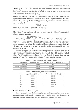
tests available in the context of age replace model. The Table 2 gives the PAE
values for different test procedures. From the Table 2, it is clear that our test
is quite efficient for the Weibull and linear failure rate alternatives.

Table 2. Pitman's asymptotic efficacy (PAE)
Distribution Proposed test Li and Xu (2008) Kayid et al. (2013)
Weibull 1.2005 1.1215 0.4822
Linear failure rate 0.8660 0.5032 0.4564
Makeham 0.2828 0.2414 2.084

Table 3. Empirical type 1 error of the test
Type 1 Error (5% level) Type 1 Error (1% level)
10 0.0635 0.0123
20 0.0540 0.0115
30 0.0518 0.0107
60 0.0516 0.0102
80 0.0511 0.0100
100 0.0504 0.0101

4. Simulation and data analysis
Next, we report a simulation study for evaluating the performance of our
asymptotic test against various alternatives. The simulation was done using R
program. Finally, we illustrate our test procedure using a real data.

5 | I S I W S C 2 0 1 9