Page 238 - Contributed Paper Session (CPS) - Volume 3

CPS2003 Bruno de S. et al.
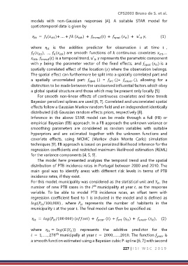
models with non-Gaussian responses [4]. A suitable STAR model for
spatiotemporal data is given by

= ( 1 )+ . . . + ( ) + () + ( ) + ′ , (1)
1

where is the additive predictor for observation at time ,
( 1 ), ..., ( ) are smooth functions of continuous covariates 1 ,...
1

, () is a temporal trend, ′ represents the parametric component

with being the parameter vector of the fixed effects, and ( ) is a

spatially correlated effect of the location () where the observation belongs.
The spatial effect can furthermore be split into a spatially correlated part and
a spatially uncorrelated part: (.) = (.)+ (.), allowing for a
distinction to be made between the unobserved influential factors which obey
a global spatial structure and those which may be present only locally [5]
For smooth non-linear effects of continuous covariates and time trends
Bayesian penalized splines are used [6, 7]. Correlated and uncorrelated spatial
effects follow a Gaussian Markov random field and an independent identically
distributed (iid) Gaussian random effects priors, respectively [8].
Inference in the above STAR model can be made through a full (FB) or
empirical Bayesian (EB) approach. In a FB approach the unknown variance or
smoothing parameters are considered as random variables with suitable
hyperpriors and are estimated together with the unknown functions and
covariate effects, using MCMC (Markov chain Monte Carlo) simulation
techniques [9]. EB approach is based on penalized likelihood inference for the
regression coefficients and restricted maximum likelihood estimation (REML)
for the variance components [4, 5, 9].
The model here presented analyzes the temporal trend and the spatial
distribution of PTB incidence rates in Portugal between 2000 and 2010. The
main goal was to identify areas with different risk levels in terms of PTB
incidence rates, if they exist.
For this model, municipality was considered as the statistical unit and , the

number of new PTB cases in the municipality at year , as the response
ℎ
variable. To be able to model PTB incidence rates, an offset term with
regression coefficient fixed to 1 is included in the model and is defined as
( /100,000) , where represents the number of habitants in the

municipality at the year . The final model can then be specified as:

= ( /100 000) () + () + ( ) + ( ), (2)

where = (( )) represents the additive predictor for the

ℎ
= 1, . . . , 278 municipally at year = 2000, . . . , 2010. The function is
a smooth function estimated using a Bayesian cubic P-spline [6, 7] with second
227 | I S I W S C 2 0 1 9