Page 150 - Contributed Paper Session (CPS) - Volume 4

CPS2160 Aye Aye Khin et al.
2.5 Granger Causality
Granger causality is a circumstance in which one time series variable
consistently and predictably changes before another variable. Granger
causality is important as it allows us to analyse which variable precedes or
leads the other variable where those leading variables are extremely useful in
order to perform forecasting purposes (Studenmund, 2017). For example, a
time series X is said to Granger-cause Y (X Granger-cause Y) when the F-test
of X to Y p-value is significantly less than 0.05 level. Granger causality is called
stationary and linear combination. It is also called cointegrated and long-term
equilibrium relationship among the variables (Studenmund, 2017).
Cointegration Analysis happens when there is a stable long-term relationship
between two variables even though individually, each variable is
nonstationary.

3. Result
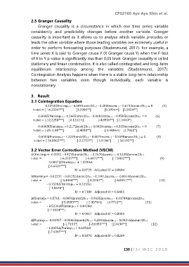
3.1 Cointegration Equation
-0.1253CHnrimpt-2 – 0.6891nrstr20t-2 – 0.2000exrmt-2 – 0.6195nrsmr20t-2 = 0 (5)
t-stat = [-14.3594***] [3.1980**] [0.3894 ] [3.2024**]
ns

-0.6985INnrimpt-1 – 1.2665nrstr20t-1 – 0.0003exrmt-1 – 0.9505nrsmr20t-1 = 0 (6)
t-stat = [-12.2258***] [0.1212 ] [-4.8910**] [-1.8443*]
ns

-0.6065USnrimpt-1 – 0.2172nrstr20t-1 – 0.0010exrmt-1 – 0.3336nrsmr20t-1 = 0 (7)
t-stat = [-20.1140***] [2.4838**] [-1.4806 ] [1.7022*]
ns

-0.0555JPnrimpt-2 – 1.2228nrstr20t-2 – 0.0071exrmt-2 – 0.5598nrsmr20t-2 = 0 (8)
t-stat = [-14.0862***] [-2.2752**] [-1.8146*] [-3.0182**]

3.2 Vector Error Correction Method (VECM)
∆CHnrimpt = -0.3592 – 0.4255∆nrstr20t-1 – 0.7670∆exrmt-1 – 0.1628∆nrsmr20t-1
t-stat = [-6.3237***] [-6.6072***] [-7.5822***] (9)
-1.0867∆CHnrimpt-1 + 1.0390εt
[-6.6531***]
R = 0.8725 Adjusted R = 0.8644
2
2

∆INnrimpt= -0.02237 – 0.01255∆nrstr20t-1 – 0.1901∆exrmt-1 – 0.0044∆nrsmr20t-1
t-stat = [-5.4984***] [-4.2230**] [-6.0891***] (10)
– 0.1520∆INnrimpt-1 + 0.3293εt
[-1.8520*]
R = 0.7180 Adjusted R = 0.6405
2
2

∆USnrimpt = 0.5761 – 0.0691∆nrstr20t-1 – 0.9635∆exrmt-1 – 0.01749∆nrsmr20t-1
t-stat = [-5.6585***] [-1.4576 ] [4.7721**] (11)
ns
- 0.5234∆USnrimpt-1 + 0.4924εt
[-7.5024***]
R = 0.9017 Adjusted R = 0.8984
2
2

∆JPnrimpt= -0.01957 – 0.00463∆nrstr20t-1 – 0.2841∆exrmt-1 – 0.00216∆nrsmr20t-1
t-stat = [-1.7153*] [-8.0355***] [2.0430**] (12)
– 1.2035∆JPnrimpt-1 + 0.6152εt
[-7.6397***]
2
R = 0.8373 Adjusted R = 0.8269
2

139 | I S I W S C 2 0 1 9