Page 159 - Contributed Paper Session (CPS) - Volume 4

CPS2164 Jonathan Hosking et al.
system matrices. For. a matrix X for which ∂logL/∂θ=tr(XA), we have ∂logL/∂X
=A ; thus, for example,
T

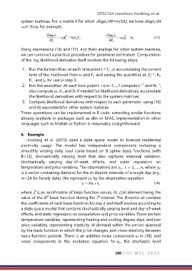
Using expressions (16) and (17), and their analogs for other system matrices,
we can construct a practical procedure for parameter estimation. Computation
of the log-likelihood derivative itself involves the following steps.

1. Run the Kalman filter, at each time point t =1,...,n accumulating the current
term of the likelihood from vt and Ft, and saving the quantities at, −1 , Kt,
Pt , and Lt for use in step 3.
2. Run the smoother. At each time point t =n,n−1,...,1 compute rt and Nt ;
−1
−1
also compute ut, ̂ t, and Dt if needed for likelihood derivatives; accumulate
the likelihood derivatives with respect to the system matrices.
3. Compute likelihood derivatives with respect to each parameter, using (16)
and its equivalentsfor other system matrices.
These operations can be implemented in R code, extending similar functions
already available in packages such as dlm or KFAS; implementation in other
languages such as Matlab or Python is reasonably straightforward.

6. Example
Hosking et al. (2013) used a state space model to forecast residential
electricity usage. The model has independent components including a
smoothly varying daily load curve based on B spline basis functions (with
B=12), stochastically varying level that also captures seasonal variation,
stochastically varying day-of-week effects, and static regression on
temperature and price variables. The observations are , = 1, … , , where

is a vector containing demand for the m disjoint intervals of a single day (e.g.,
m=24 for hourly data). We represent by the observation equation

where Z is an m×B matrix of basis function values, its (i,b) element being the
th
th
value of the b basis function during the i interval. The B-vector αt contains
the coefficients of each basis function for day t, and itself evolves according to
a state space model that contains stochastically varying level and day-of-week
effects, and static regression on temperature and price variables. There are two
temperature variables, representing heating and cooling degree days, and two
price variables, representing elasticity of demand within the period spanned
by the basis function in which the price changes, and cross-elasticity between
basis-function periods. There is an additive noise component εt in (18), and
noise components in the evolution equation for , the stochastic level

148 | I S I W S C 2 0 1 9