Page 156 - Contributed Paper Session (CPS) - Volume 4

CPS2164 Jonathan Hosking et al.
forecasting models. They are suitable for modeling and forecasting many kinds
of time series data.
Inference for state space models commonly uses Kalman filtering and
smoothing iterations, which provide conditional distributions of the state
vector αt given observations up to time t or all observations in t =1,...,n, and
can also be used to forecast future observations. When used in practice, state
space models typically include model parameters that must be estimated from
observed data. Maximum-likelihood estimation is commonly used, with the
likelihood being maximized by optimization procedures that use numerical
derivatives of the likelihood function. The optimization step can be greatly
accelerated by the use of analytical derivatives.
In this paper we present a new analytical expression for the log-likelihood
derivative, eq. (14) below. This expression can be computed using quantities
that are routinely computed during the Kalman filtering and smoothing
iterations, and involve no additional iterations. To the best of our knowledge
all previously published expressions either require further iterations or do not
cover all possibilities of the state space model Our result makes it
straightforward to construct an optimization method based on gradient
descent: in Sections 5 and 6 we outline the construction of such a method and
illustrate its performance.

2. Filtering and smoothing
Inferential procedures for state space models commonly include filtering
and smoothing. Let Yt denote the information available at time t, i.e., the data
{y1,...,yt}. The Kalman filter computes estimates of the states at time t based
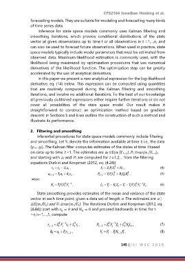
on data up to time t −1. The estimates are at ≡E(αt |Yt−1), Pt ≡var(αt |Yt−1),
and starting with a1 and P1 are computed for t =1,2,... from the filtering
equations Durbin and Koopman (2012, eq. (4.24))

State smoothing provides estimates of the mean and variance of the state
vector at each time point, given a data set of length n. The estimates are αˆt
≡E(αt |Yn) and Vt ≡var(αt |Yn). The iterations Durbin and Koopman (2012, eq.
(4.44)) start with = 0 and = 0 and proceed backwards in time: for t

=n,n−1,...,1, compute

145 | I S I W S C 2 0 1 9