Page 141 - Contributed Paper Session (CPS) - Volume 7

CPS2048 Md Zobaer H. et al.
Where, for each DMU s is output observation, m is input observation, r is ℎ
ℎ
ℎ
ℎ
output, i is input, is output for time period t, is input for

time period t, n is DMU observation, j is DMU, is no-negative scalar, is
ℎ

ℎ input for nth DMU, is ℎ output for ℎ DMU, is a scalar

representing the value of efficiency score for each DMU. Similar method is
applied for DMUs. To measure the technical efficiency, the software DEAP
ℎ
version 2.1 is used.
SFA
The production theory is proposed by Cobb and Douglas (1928) and
named “Cobb Douglass production theory”. He develops the production
theory by using of labour, capital, production, value, and wages for the
manufacturing firms. In order to measure statistical noise, Aigner et al. (1977)
added symmetric error term to the deterministic frontier. The model expressed
as:
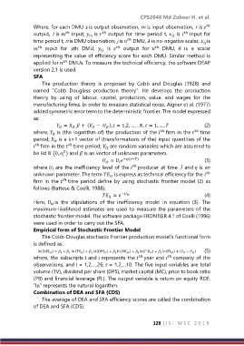
= + ( − ), = 1,2, … . . , = 1, … , (2)

ℎ
ℎ
where, is (the logarithm of) the production of the firm in the time

period; is a k×1 vector of (transformations of the) input quantities of the

ℎ firm in the ℎ time period; are random variables which are assumed to

2
be iid (0, ) and is an vector of unknown parameters.

= −(−) (3)

where are the inefficiency level of the ℎ producer at time T and is an

unknown parameter. The term is express as technical efficiency for the ℎ

firm in the ℎ time period define by using stochastic frontier model (2) as
follows (Battese & Coelli, 1988):
= − (4)

Here, is the stipulations of the inefficiency model in equation (3). The

maximum-likelihood estimates are used to measure the parameters of the
stochastic frontier model. The software package FRONTIER 4.1 of Coelli (1996)
were used in order to carry out the SFA.
Empirical form of Stochastic Frontier Model
The Cobb-Douglas stochastic frontier production model’s functional form
is defined as:
) ) ) ) ) ) ) (5)
ln(ROE = 0 + 1 ln(TV + 2 ln(DPS + 3 ln(MC + 4 ln(P + 5 ln(FL + ( −
where, the subscripts and represents the ℎ year and ℎ company of the
observations, and = 1,2,….26; = 1,2,…10. The five input variables are total
volume (TV), dividend per share (DPS), market capital (MC), price to book ratio
(PB) and financial leverage (FL). The output variable is return on equity ROE.
“ln” represents the natural logarithm.
Combination of DEA and SFA (CDS)
The average of DEA and SFA efficiency scores are called the combination
of DEA and SFA (CDS).

128 | I S I W S C 2 0 1 9