Page 164 - Contributed Paper Session (CPS) - Volume 7

CPS2051 Mentje G. et al.
consistency, we put tildes on all estimates of distribution functions which
involve use of the scenario assessments.
Next, () can be modelled by the (; , , ) distribution. For ease

of explanation, suppose we have actual scenario assessments ̃ , ̃ and ̃ 100
7
20
and thus take = 7 and estimate by ̃ . Substituting these scenario

7

assessments into ( ) = 1 − ; with = 7, = 20, 100 yields two equations

)
)
(̃ 20 = GDP(̃ 20 ; , ξ, ̃ 7 ) = 0.65 and (̃ 100 = GDP(̃ 100 ; , ξ, ̃ 7 ) = 0.93 (3)
that can be solved to obtain estimates of the parameters and in the GPD
that are based on the scenario assessments. Some algebra shows that a
solution exists only if ̃ 100 − ̃ 7 > 2.533. This fact should be borne in mind when
̃ 20 − ̃ 7
the experts do their assessments.
With more than three scenario assessments, fitting techniques can be
based on (3) which links the quantiles of the GPD to the scenario assessments.
An example would be to minimize ∑ |GDP(̃ ;, ξ, ̃ ) − (1 − /)| .Other
7

possibilities include a weighted version of the sum of deviations in this
expression or deviation measures comparing the GPD quantiles directly to the
assessments. Whichever route we follow, we denote the final estimate of

̃
() by () All these ingredients can now be substituted into (2) to yield

̃
the estimate () of (), namely
1 1 (4)
̂ ̃
̃
̃
̂
() = ( − ) () + ().
7 7
When using the GPD 1-in- years integration approach to model the
severity distribution in the LDA, we realised that the 99.9% VaR of the
aggregate distribution is almost exclusively determined by the scenario
assessments and their reliability greatly affects the reliability of the VaR
estimate. The fitted distribution has little effect on the VaR estimates. However,
if the assessments are supplied by experts and not oracles, this may render
undesirable results. The challenge is therefore to find a way of integrating the
historical data and scenario assessments such that both sets of information
are adequately utilised in the process.
2.5 Venter’s approach
A retired colleague, Hennie Venter suggested that, given the quantiles
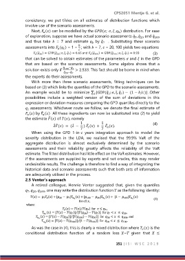
, , 100 , one may write the distribution function as the following identity:
7
20

As was the case in (4), this is clearly a mixed distribution where () is the

conditional distribution function of a random loss ~ given that ≤

151 | I S I W S C 2 0 1 9