Page 165 - Contributed Paper Session (CPS) - Volume 7

CPS2051 Mentje G. et al.
, () the conditional distribution function given that < ≤
7
7
1
, () the conditional distribution function given that 20 < ≤ 100
2
20
and () is the conditional distribution function given that > 100 .
3
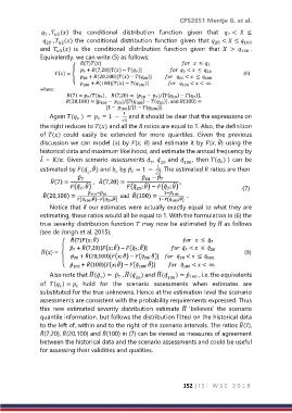
Equivalently, we can write (5) as follows:

1
Again ( ) = = 1 − and it should be clear that the expressions on

the right reduces to () and all the ratios are equal to 1. Also, the definition
of () could easily be extended for more quantiles. Given the previous
̂
discussion we can model () by (, ) and estimate it by (, ) using the
historical data and maximum likelihood, and estimate the annual frequency by
̂
= /. Given scenario assessments , and 100 , then ( ) ) can be

20
7
1
̂
estimated by ( , ) and by = 1 − . The estimated ratios are then
̂

Notice that if our estimates were actually exactly equal to what they are
estimating, these ratios would all be equal to 1. With the formulation in (6) the
̃
true severity distribution function may now be estimated by as follows
(see de Jongh et al. 2015):

̃
̃
̃
Also note that ( ) = , ( ) and ( ) = , i.e. the equivalents
7 7 20 100 100
of ( ) = hold for the scenario assessments when estimates are

substituted for the true unknowns. Hence at the estimation level the scenario
assessments are consistent with the probability requirements expressed. Thus
̃
this new estimated severity distribution estimate ‘believes’ the scenario
quantile information, but follows the distribution fitted on the historical data
̃
to the left of, within and to the right of the scenario intervals. The ratios (7),
(7,20), (20,100) and (100) in (7) can be viewed as measures of agreement
̃
̃
̃
between the historical data and the scenario assessments and could be useful
for assessing their validities and qualities.

152 | I S I W S C 2 0 1 9