Page 60 - Contributed Paper Session (CPS) - Volume 8
P. 60
CPS2184 M Lutfor Rahman
time spent together/relation (hours in 12 weeks), type of contacts
(Co-habitant/ family/ friend/ work colleague/ known/ teacher/ patient/ others;
grouped as casual/household), sleep together (Yes/No), eat together
2
2
(Yes/No), size of exposure site (<12m - “small”, ≥ 12 m - “large”), location of
contact (Car/ Bedroom/ Living room/Dining room/ Restaurant/ Open space/
coffee/ Other), ventilation facility of the exposure site (Yes/No). As each of the
index patients are connected to several contacts, a hierarchical logit model can
be employed to model the infection status considering risk factors. The
hierarchical models are designed to handle mutual dependence among data
points [23]. The last one is network logistic regression which could be more
appropriate but also more complicated to implement in this study and as it is
less known and used, some basic theoretical details are presented here and
contextualized in our case-study.
Some network concepts: Metrics and Logistic Regression
In the present study, as it is one step network, i.e. the network of index-
contact exists only, but no index-index or no contact-contact relations. For this
reason, many of the social networks analyzing tools, though exist, do not carry
meaningful interpretations and therefore, they are not explored for the current
data. However, implementation of network logistic regression might be a
realistic tool for studying any infectious disease including the current TB index-
contact network. Because, network logistic regression considers the structural
position of the TB patients interacting contacts as well as cofactors associated
with index and contacts.
The logistic network regression framework is a simple basis for the
modelling of joint edge/vertex dynamics with various orders of temporal
dependence (Almquist and Butts, 2014). The models can be associated with
dynamic network logistic regression or conventional cross-sectional network
logistic regression. Given a random graph G on support Ψ, Almquist and Butts
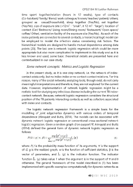
(2014) defined the general form of dynamic network logistic regression as
follows:
where P(.) is the probability mass function of its arguments, is the support
of G, g is the realized graph, w is the function of sufficient statistics, is the
vector of parameters, and (g) is the indicator function. The indicator
function (g) takes value 1 when the argument is in the support of and 0
otherwise. The general framework of the model described in (1) has been
implemented with specific examples computationally for dynamic networks as
49 | I S I W S C 2 0 1 9

