Page 74 - Contributed Paper Session (CPS) - Volume 8

CPS2187 Lukasz Widla-Domaradzki
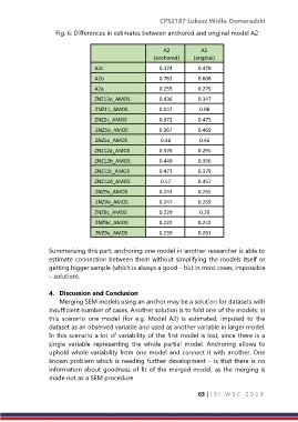
Fig. 6: Differences in estimates between anchored and original model A2

A2 A2

(anchored) (original)
A2c 0.374 0.478
A2b 0.763 0.608

A2a 0.255 0.279
ZNZ12e_AMOS 0.436 0.347
ZNZ11_AMOS 0.047 0.06
ZNZ5c_AMOS 0.372 0.475

ZNZ5b_AMOS 0.367 0.469
ZNZ5a_AMOS 0.36 0.46
ZNZ12a_AMOS 0.376 0.295
ZNZ12b_AMOS 0.449 0.356
ZNZ12c_AMOS 0.473 0.379

ZNZ12d_AMOS 0.57 0.457
ZNZ9a_AMOS 0.243 0.265
ZNZ9b_AMOS 0.247 0.269
ZNZ9c_AMOS 0.229 0.25

ZNZ9d_AMOS 0.222 0.242
ZNZ9e_AMOS 0.239 0.261

Summarizing this part, anchoring one model in another researcher is able to
estimate connection between them without simplifying the models itself or
getting bigger sample (which is always a good – but in most cases, impossible
– solution).

4. Discussion and Conclusion
Merging SEM models using an anchor may be a solution for datasets with
insufficient number of cases. Another solution is to fold one of the models: in
this scenario one model (for e.g. Model A2) is estimated, imputed to the
dataset as an observed variable and used as another variable in larger model.
In this scenario a lot of variability of the first model is lost, since there is a
single variable representing the whole partial model. Anchoring allows to
uphold whole variability from one model and connect it with another. One
known problem which is needing further development – is that there is no
information about goodness of fit of the merged model, as the merging is
made not as a SEM procedure

63 | I S I W S C 2 0 1 9