Page 107 - Contributed Paper Session (CPS) - Volume 6

CPS1837 Qiguang Dong et al.
Xu,1997). Hence, both issues inherent in the high frequency observations are
considered in this paper.
In the specification of model structure, Barkoulas and Baum (1997) first use
the ARFIMA model structure to forecast the Eurocurrency return series and
show that the ARFIMA model can improve of the forecasts. Unlike the
autocorrelation process decays exponentially in the ARMA model, it decays
hyperbolically which can be more slowly in the ARFIMA model. Besides,
Andersen et al. (2008) find that the out-of-sample forecasts based on ARFIMA
model are performed better than other long memory models, such as
FIGARCH, FIEGARCH. In addition, Kanellopoulou and Panas (2008) argue that
the ARFIMA models are strictly based on the assumptions of no conditional
heteroscedasticity and normal distributions, otherwise the forecasts will be
biased. However, previous literature confirms that the volatility of financial
assets violates both assumptions. Researchers use the logarithm-transformed
realized variance, namely LnRV, instead of RV in the model specification.
Though LnRV series are more approximate normal distribution than RV series.
Hence, this paper considered these problems during the model specification
by combining GARCH family models and non-normal distributions. In the
evaluation of models predictive ability, Hansen and Lunde (2005) introduced
Superior Predictive Ability (SPA) test based on the bootstrap method, which
use a set of loss functions to deliver the optimal models with respect to a
given set of loss functions. SPA test needs to set benchmark model at first,
then the other models are compared to the benchmark model so that models
that produce better forecasts are preferred. However, the procedure may
bring two problems: first, the comparing procedure may not deliver a unique
result; second, sometimes it is not trivial to asses which model clearly
outperforms each other. For overcoming the deficiencies of SPA test, Hansen,
Lunde and Nason (2011) further introduced a new test, the Model Confidence
Set (MCS) test. MCS test permits to construct a set of “superior” models, and
can directly evaluate and compare the models predictive ability in the set.

2. Methodology
In the specification of volatility forecasting model, Andersen et al. (2003)
find that the variance pattern of financial asset can be described as Gaussian
dynamic process, and the RV series shows long memory features. Based on
this, this paper chooses the long term ARFIMA to construct the empirical
model.

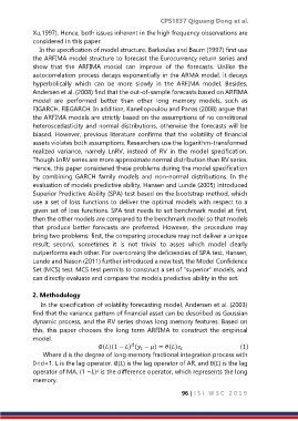
∅()(1 − ) ( − ) = () (1)

Where d is the degree of long memory fractional integration process with
0<d<1. L is the lag operator. ∅() is the lag operator of AR, and θ() is the lag
operator of MA. (1 −) is the difference operator, which represents the long

memory.

96 | I S I W S C 2 0 1 9