Page 198 - Contributed Paper Session (CPS) - Volume 6

CPS1881 Mike S.C. et al.
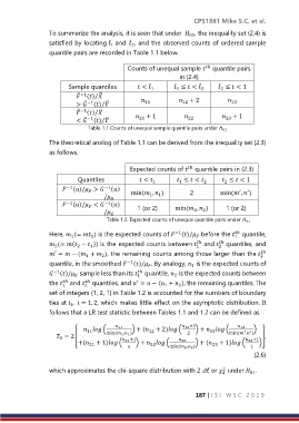
To summarize the analysis, it is seen that under , the inequality set (2.4) is
01
satisfied by locating ̂ and ̂ , and the observed counts of ordered sample
2
1
quantile pairs are recorded in Table 1.1 below.

Counts of unequal sample quantile pairs
ℎ
in (2.4)
Sample quantiles < ̂ ̂ ≤ < ̂ ̂ ≤ < 1
2
2
1
1
̂
̅
⁄
−1 () + 2
̅
⁄
> ̂ −1 () 11 12 13
̂
̅
⁄
−1 () + 1 + 1
̅
⁄
< ̂ −1 () 21 22 23
Table 1.1 Counts of unequal sample quantile pairs under 01
The theoretical analog of Table 1.1 can be derived from the inequality set (2.3)
as follows.
Expected counts of quantile pairs in (2.3)
ℎ
Quantiles < ≤ < ≤ < 1
1
2
2
1
−1 ()/ > −1 () min ( , ) 2 min ( , )
′
′

/ 1 1

−1 ()/ < −1 () 1 (or 2) min ( , ) 1 (or 2)

/ 2 2

Table 1.2. Expected counts of unequal quantile pairs under 01
ℎ
Here, (= ) is the expected counts of −1 ()/ before the quantile,
1
1
1

(= ( − )) is the expected counts between and quantiles, and
ℎ
ℎ
2
2
1
1
2
′
= − ( + ), the remaining counts among those larger than the
ℎ
2
1
2
quantile, in the smoothed −1 ()/ . By analogy, is the expected counts of
1

ℎ
−1 ()/ sample less than its quantile, is the expected counts between

1
2
ℎ
ℎ
the and quantiles, and = − ( + ), the remaining quantiles. The
′
2
2
1
1
set of integers {1, 2, 1} in Table 1.2 is accounted for the numbers of boundary
ties at , = 1, 2, which makes little effect on the asymptotic distribution. It

follows that a LR test statistic between Tables 1.1 and 1.2 can be defined as
( 11 ) + ( 12 + 2) ( 12 +2 ) + ( 13 ′ ′ )
11
13
= 2 [ min ( 1 , 1 ) 2 min ( , ) ],
0
21 +1
23 +1
22
+( 21 + 1) ( 1 ) + ( min ( 2 , 2 ) ) + ( 23 + 1) ( 1 )
22
(2.6)
2
which approximates the chi-square distribution with 2 df, or under .
01
2
187 | I S I W S C 2 0 1 9