Page 43 - Special Topic Session (STS) - Volume 2

STS452 Nobuhiro O.
: a scalar, the number of urban workers
: a scalar, the number of rural workers
: a scalar, the level of labour supply

If the matrix is partitioned with the economic and demographic activity, then
it can be converted to a simple form of the equation as follows:
− −
[ ] [ ] = [ ]
−

̇
̇
where = [ℎ ℎ ], = [ ], = [ 1 0 ]. In addition, = [ ] is defined as

1
1
0
0
the number of urban and rural workers, = [ ] is the number of commuting

1
workers from rural areas , which is assumed to be an imbalance and therefore
set at zero, and the number of active economic population or labour supply
of the country. The equation can then be rewritten as:
22
− − −1 11 12 ( + ) 22

[ ] = [ − ] [ ] = [ 21 22 ] [ ] = [ 22 ] [ ]
22

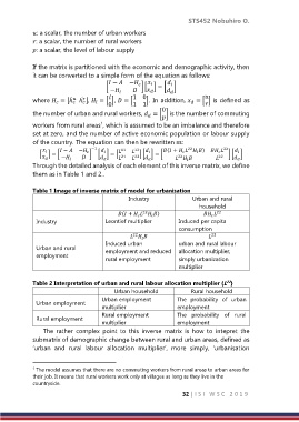
Through the detailed analysis of each element of this inverse matrix, we define
them as in Table 1 and 2..

Table 1 Image of inverse matrix of model for urbanisation
Industry Urban and rural
household
22
( + )
22

Industry Leontief multiplier Induced per capita
consumption

22
22

Induced urban urban and rural labour
Urban and rural employment and reduced allocation multiplier,
employment
rural employment simply urbanization
multiplier

22
Table 2 Interpretation of urban and rural labour allocation multiplier (L )
Urban household Rural household
Urban employment The probability of urban
Urban employment
multiplier employment
Rural employment The probability of rural
Rural employment
multiplier employment
The rather complex point to this inverse matrix is how to intepret the
submatrix of demographic change between rural and urban areas, defined as
‘urban and rural labour allocation multiplier’, more simply, ‘urbanisation

1 The model assumes that there are no commuting workers from rural areas to urban areas for
their job. It means that rural workers work only at villages as long as they live in the
countryside.
32 | I S I W S C 2 0 1 9