Page 262 - Special Topic Session (STS) - Volume 3

STS543 Veronica B. B. et al.
commitment. The study considers a specification that considers the sum of
one lag to four quarter lag effects to capture the total effects in t as seen in
equation 1. In the exercise, the propagation of the effects of changes in
domestic macroprudential policy to changes in loan commitment is significant
across different regression models up to four quarters.
Do responses to a macroprudential shock differ by type of banks? This
section looks at the difference between domestic U/KBs and TBs responses to
a macroprudential shock. In the database, there are 101 respondent banks, 38
of which are U/KBs and the remaining 63 are TBs. However, only 56 banks
consistently reported residential property loans granted on a quarterly basis
from the first quarter of 2014 to the fourth quarter of 2017. Hence, data of
these 56 banks are used in all regression models.
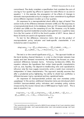
To test for the difference, interaction terms that are the product of
macroprudential policy indicator and bank-specific characteristic X are
included as seen in equation 2,

∆ log , = + ∑ =1 ∆ log ,− + ∑ =1 ∆ − + ,−1 +

∑ ∆ ∗ + + (eq. 2)
=1 − ,−1 , ,

The test is on the overall significance of ∑ =1 . This approach builds on
the bank lending channel literature. In order to discriminate between loan
supply and loan demand movements, the literature has focused on cross-
sectional differences between banks. Following Gambacorta (2005), this
equation relieson the hypothesis that certain bank-specific characteristics,
such as, size, liquidity, the deposit-to-totalfunding ratio and capitalization,
influence only the loan supply movements, while a bank’s loan demand is
independent of these characteristics. This approach basically assumes that
after a prudential policy tightening, the ability to shield loan portfolios is
different between highly-capitalized and less-capitalized banks.
Do responses to macroprudential policies vary over monetary policy
conditions? In this section, additional interaction terms are introduced which
combine macroprudential policy indicators and monetary policy actions
2
(measured by the neutral interest rate or NRR based on Taylor rule ). This is
seen in equation 3 as,

∆ log , = + ∑ =1 ∆ log ,− + ∑ =1 ∆ − + ∑ +

=0

−
∑ ∆ ∗ + + +
=1 − −1 ,−1 , ,
(eq. 3)

2 The neutral interest rate (NRR) is derived as NRR=(10-year average of real 1-year secondary rates)-
((real 1-year secondary rates - real 5-year secondary rates) - (real 1-year secondary average - real 5-year
secondary average)).

251 | I S I W S C 2 0 1 9