Page 354 - Special Topic Session (STS) - Volume 3

STS550 Angelia L. Grant et al.
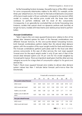
As the forecasting horizon increases, the performance of the AR(2) models
for some components deteriorates relative to the AIDS. For example, at the
three-year-ahead horizon, the forecast for the fuels and lubricants component
of the benchmark model is 53 per cent better compared to the standard AR(2)
model. In contrast, the relative price model with the linear time trend
continues to perform relatively well for most of the components.
Consequently, it can generally be concluded that, at shorter forecasting time
horizons, models that capture short-run dynamics perform well, but that, at
longer horizons, models with trend terms and relative prices tend to perform
better.

Forecast Combinations
Table 2 reports the root mean squared forecast error relative to that of the
almost ideal demand system for both of the forecast combinations over
different forecast horizons. At the one-quarter-ahead forecasting horizon,
both forecast combinations perform better than the almost ideal demand
system, with the exception of the equal weight model for fuels and lubricants.
The forecast combinations perform particularly well for the food and other
services components. In the case of other services, the root mean squared
forecast error for the equal weight model is only 25 per cent of that of the
almost ideal demand system and 19 per cent for the model weighted by
forecast performance. This is an important result given that the other services
category accounts for a large share of consumption subject to the goods and
services tax.
Table 1: Root mean squared forecast error relative to almost ideal demand
system (values less than 1 indicate better forecast performance than the
benchmark).

Household consumption components*

(a) (b) (c) (d) (e) (f) (g) (h) (i)
One-quarter-ahead forecast
AR(2) model 0.21 0.40 0.23 0.23 0.17 0.38 0.82 0.76 0.21

AR(2) model with trend 0.22 0.45 0.22 0.21 0.16 0.36 0.74 0.71 0.16
Relative price model 0.81 0.85 1.30 1.25 1.43 0.97 3.71 1.11 0.57

Relative price model with 0.75 1.08 0.32 0.33 0.45 0.81 1.06 0.80 0.17
trend

One-year-ahead forecast
AR(2) model 0.37 0.87 0.72 0.29 0.34 0.81 1.77 1.56 0.33
AR(2) model with trend 0.45 1.09 0.70 0.30 0.32 0.78 1.58 1.44 0.12

343 | I S I W S C 2 0 1 9