Page 355 - Special Topic Session (STS) - Volume 3

STS550 Angelia L. Grant et al.

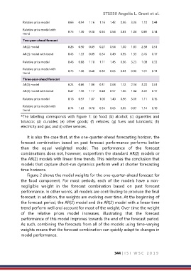
Relative price model 0.66 0.94 1.16 1.16 1.42 0.96 3.36 1.10 0.44
Relative price model with 0.75 1.30 0.38 0.34 0.54 0.83 1.04 0.89 0.14
trend
Two-year-ahead forecast
AR(2) model 0.26 0.90 0.89 0.27 0.54 1.00 1.83 2.58 0.51
AR(2) model with trend 0.43 1.33 0.89 0.34 0.49 0.95 1.33 2.45 0.17

Relative price model 0.46 0.88 1.10 1.11 1.45 0.96 3.23 1.08 0.33
Relative price model with 0.75 1.36 0.40 0.32 0.65 0.83 0.96 1.01 0.11
trend
Three-year-ahead forecast
AR(2) model 0.24 0.86 1.06 0.31 0.68 1.12 2.14 3.20 0.61
AR(2) model with trend 0.47 1.56 1.17 0.40 0.57 1.06 1.04 3.22 0.17
Relative price model 0.18 0.97 1.07 1.03 1.40 0.96 3.16 1.11 0.15

Relative price model with 0.74 1.63 0.78 0.34 0.65 0.85 0.87 1.14 0.10
trend
*The labelling corresponds with Figure 1: (a) food; (b) alcohol; (c) cigarettes and
tobacco; (d) durables; (e) other goods; (f) vehicles; (g) fuels and lubricants; (h)
electricity and gas; and (i) other services.

It is also the case that, at the one-quarter-ahead forecasting horizon, the
forecast combination based on past forecast performance performs better
than the equal weighted model. The performance of the forecast
combinations does not, however, outperform the standard AR(2) models or
the AR(2) models with linear time trends. This reinforces the conclusion that
models that capture short-run dynamics perform well at shorter forecasting
time horizons.
Figure 2 shows the model weights for the one-quarter-ahead forecast for
the food component. For most periods, each of the models have a non-
negligible weight in the forecast combination based on past forecast
performance. In other words, all models are contributing to produce the final
forecast. In addition, the weights are evolving over time. At the beginning of
the forecast period, the AR(2) model and the AR(2) model with a linear time
trend perform well and account for most of the weight. Over time the weight
of the relative prices model increases, illustrating that the forecast
performance of this model improves towards the end of the forecast period.
As such, combining the forecasts from all of the models using time-varying
weights means that the forecast combination can quickly adapt to changes in
model performance.

344 | I S I W S C 2 0 1 9