Page 356 - Special Topic Session (STS) - Volume 3

STS550 Angelia L. Grant et al.

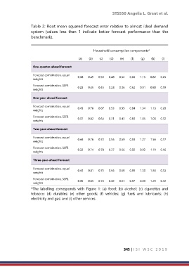
Table 2: Root mean squared forecast error relative to almost ideal demand
system (values less than 1 indicate better forecast performance than the
benchmark).

Household consumption components*

(a) (b) (c) (d) (e) (f) (g) (h) (i)

One-quarter-ahead forecast

Forecast combination, equal 0.38 0.49 0.53 0.48 0.52 0.66 1.15 0.82 0.25
weights
Forecast combination, SSFE
weights 0.22 0.45 0.45 0.24 0.36 0.52 0.91 0.80 0.19

One-year-ahead forecast

Forecast combination, equal
weights 0.45 0.76 0.67 0.53 0.55 0.84 1.34 1.13 0.20
Forecast combination, SSFE
weights 0.37 0.82 0.64 0.31 0.43 0.83 1.05 1.03 0.12

Two-year-ahead forecast

Forecast combination, equal
weights 0.44 0.76 0.72 0.55 0.59 0.93 1.27 1.56 0.17
Forecast combination, SSFE
weights 0.32 0.74 0.70 0.37 0.56 0.92 0.92 1.19 0.16

Three-year-ahead forecast

Forecast combination, equal
weights 0.44 0.81 0.75 0.56 0.58 0.99 1.30 1.84 0.12
Forecast combination, SSFE 0.30 0.65 0.73 0.42 0.61 0.97 0.99 1.29 0.12
weights
*The labelling corresponds with Figure 1: (a) food; (b) alcohol; (c) cigarettes and
tobacco; (d) durables; (e) other goods; (f) vehicles; (g) fuels and lubricants; (h)
electricity and gas; and (i) other services.

345 | I S I W S C 2 0 1 9