Page 78 - Contributed Paper Session (CPS) - Volume 1

CPS1085 Manoj C.
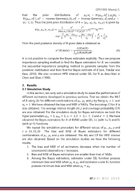
that the prior distributions of | ∼ ( , ), | ∼
2
1
01
1
1
2
2
2
2
2
( , ), ∼ Inverse Gamma(, ), ∼ Inverse Gamma(, ) and ∼
2
1
2
02
(−1, 1). Thus the joint prior distribution of = ( , , , , ) is given by
2
1
2
1

1
( , , , , ) = 1 −2−1 −2−1

1
2
2
1
2
2 Γ()2 −1 Γ()2 −1
1 2
−1 − − 02 2
2
1
{( 01 2 ) + + }.
) + (
2 1 2 1 2 2 2

Then the joint posterior density of θ given data is obtained as

()()
∗
(|) = . (6)
∫ ()()

It is not possible to compute the Bayes estimates explicitly. Thus we propose
importance sampling method to find the Bayes estimators for . we consider
the sequential importance sampling method to generate samples from the
posterior distribution and then find the Bayes estimate of (see, Tokdar and
Kass, 2010). We also construct HPD interval under SEL for R as described in
Chen and Shao (1999).

3. Results
3.1 Simulation Study
In this section, we carry out a simulation study to asses the performance of
different estimators developed in previous sections. First we obtain the MLE
of using (5) for different combinations of , and by fixing = 1 and
2
1
1
= 1. We have obtained the bias and MSE of MLEs. The bootstrap CI for is
2
also obtained. The average interval length (AIL) and coverage probability (CP)
are also obtained. For the simulation study for Bayes estimators we took the
hyper parameters 01 = 2, 02 = 2, = 2, = 2, = 2 and = 2. We have
obtained the Bayes estimators for of BVND under SEL, LL (with h=1) and EL
(with q=1) functions.
We repeat the simulation procedure for different values of , , and
2
1
= 10, 15, 20 . The bias and MSE of Bayes estimators for different
combinations of , and are obtained. The AIL and CP for HPD interval
2
1
are also obtained. Based on the simulation studies we have the following
results.
1. The bias and MSE of all estimators decrease when the number of
uncensored observations increases.
2. Bias and MSE of Bayes estimators are smaller than that of MLEs.
3. Among the Bayes estimators, estimator under SEL function possess
minimum bias and MSE when ≠ and estimator under EL function
2
1
possess minimum bias and MSE when = .
2
1
67 | I S I W S C 2 0 1 9