Page 83 - Contributed Paper Session (CPS) - Volume 1

CPS1110 Selamawit M. et al.
Posterior model
The posterior pdf constitute the solution to the Bayesian inversion and it
is defined by the prior pdf and the likelihood function. It can be presented as

(|d) = const × ( | ) × ( ) ∏ ( | −1 )
1

∈ −1
= const × ( | )( ) × ∏ ( | )( | −1 )

1
1
1

∈ −1
= ( |d) ∏ ( | −1 , d : ) (5)
1

∈ −1

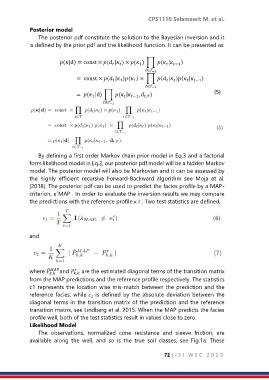
By defining a first order Markov chain prior model in Eq.3 and a factorial
form likelihood model in Eq.2, our posterior pdf model will be a hidden Markov
model. The posterior model will also be Markovian and it can be assessed by
the highly efficient recursive Forward-Backward algorithm see Moja et al.
(2018). The posterior pdf can be used to predict the facies profile by a MAP-
criterion, κˆMAP . In order to evaluate the inversion results we may compare
the predictions with the reference profile κ r . Two test statistics are defined,

and

̂

where , and are the estimated diagonal terms of the transition matrix
,
from the MAP predictions and the reference profile respectively. The statistics
c1 represents the location wise mis-match between the prediction and the
reference facies, while is defined by the absolute deviation between the
2
diagonal terms in the transition matrix of the prediction and the reference
transition matrix, see Lindberg et al. 2015. When the MAP predicts the facies
profile well, both of the test statistics result in values close to zero.
Likelihood Model
The observations, normalized cone resistance and sleeve friction, are
available along the well, and so is the true soil classes, see Fig.1a. These

72 | I S I W S C 2 0 1 9