Page 97 - Contributed Paper Session (CPS) - Volume 1
P. 97

CPS1158 Varun A. et al.
                                                                     th
                                                                                      th
            lag considered and rij is the threshold parameter of the j  regime of the i
            break  point  constitute  a  partition  on  the  real  line  and  satisfy
             − = r i0  r i1    r  i ik  =   .   The   locations  of   structural   breaks   are
             0  = T   T    T =  T  that  partition  the  time  series  into  TAR  models.  The
                            m
                    1
                 0
            number of structural breaks (m) having partition in such a way that each break
            segment having ki regimes TAR model with delay parameter di. The error term
              is independent and identically normal distributed random variable with
              (ij
               )
             e
              t
            mean zero and unknown variance . Also, TAR model coefficients  and
                                                                                
                                                2
                                                                                 (ij
                                                                                  )
                                               ij
                                                                                l
            lags order   are also different with respect to change in threshold and delay
                        p

                         ij
            parameter as well as the presence of break points. In time series, sequential
            observations  is  valuable  for  making  effective  statistical  inference  so
            reorganized the MB-TAR generating observations in a group of each regimes
            for a particular break interval. This separation appears in an order form and
                                                                                      th
            does not need to know the threshold value. Let πij be the time index of the j
                                    th
            smallest observation in i  break point in this series. Then, each regime has (sij-
            sij-1)  observations  from  (yp+1-d,  yp+2-d,…,  yTi-d)  where  p=max(pij;  i=1,2,…,m;
            j=1,2,…,ki). Therefore, we can rewrite the model (1) as given by
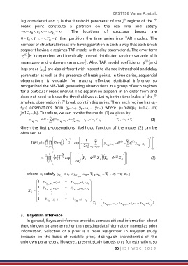
                            p ij  ( ij)  ( ij)                                    (2)
                         ij)
                         (
                      = 
                            
                           +
                   y  w + d i  l =1  l  y  w + d i − l + e  w +  d i  ij s −1  w ij   ij s  i T −1  ij s   i T  (2)
                                          ij
                                  ij
                   ij

            Given the first p-observations, likelihood function of the model (2)  can be

            obtained as
                                    s ij  −s ij −1                              2   
                          m k i
                   ( L   y |  )     (2 ij 2 ) −  2  exp −  1  s ij   y  − ( ij)  −  p ij  l ( ij) y   −l      
                        =
                                                                       
                                                     
                                                          
                          = i 1  = j   1     2 ij 2  w ij  =s ij −1  +1   w ij  +d i  = l 1  w ij  +d i     
                                                                                    
                                  n ij                               
                          m k i    2  −   1        ( ij)  '    ( ij)  
                             ij     −    ( Y ij  −  X ij  )( Y ij  −  X ij )  (3)
                              ( ) 2 exp
                         i 1           2 ij 2                       
                                        
                          = = j 1

                where  sij satisfy  y   r   y  s ,  =    T  s ,  =  T   , nij =sij-sij-1;
                                   ij s   ij  ij s   + 1  i0  1 - i  ik i  i
                     1  y             y         
                          ij s  −1 +1 +d i  −1  ij s   −1 +1 +d i  − p ij  
                     1  y    +d  −1    y   +d  − p  
                X ij  =   ij s   −1  +2  i  ij s   −1  +2  i  ij  
                                             
                      1  y             y        
                           ij s   +d i  −1  ij s   +d i − p ij    Y ij  =    y  s  +1  +d i  ,  y  s  +2 +d i  , ,  y  s  +d i   ;
                                                                                    
                                                        
                                                                                    
                                                            ij  −1  ij  −1      ij
            3.  Bayesian Inference
                In general, Bayesian inference provides some additional information about
            the unknown parameter rather than existing data information named as prior
            information.  Selection  of  a  prior  is  a  main  assignment  in  Bayesian  study
            because  on  the  basis  of  suitable  prior,  distinguish  characteristic  of  the
            unknown parameters. However, present study targets only for estimation, so
                                                                86 | I S I   W S C   2 0 1 9
   92   93   94   95   96   97   98   99   100   101   102